Building a computational graph: part 1
This is the first post in a series on computational graphs. You can go to the next post or skip ahead to the third post.
If you’d like to see what we are working towards in these posts, here is the Github link:
Computation graphs have many uses. Here I’ll be presenting it as they used for autodifferentiation.
For this post, I’ll assume you have some familiarity with backpropagation and autodifferentiation (also known as autodiff).
Many packages exist to do autodiff. One well-known one for Python is the autograd package. Autodidact package is a somewhat simplified version of autograd. The computational graph we’ll be building in this and future posts is based off the one used in autograd/autodidact.
What are we looking for? Link to heading
Say we have a function $f$ we want to differentiate that takes some number of arguments: one, two, three… however many. Our aim is to find $df/dv$, where $v$ is one of these arguments to $f$.
For example, this is a function with two variables: $x$ and $y$. $$f(x,y) = \log(x^2) + y^2 + xy$$
In python:
def f(x,y): return np.log(x**2) + y**2 + x*y
How do we find the gradient? It depends on what autodiff package you are using.
The autograd/autodidact packages create a function grad that takes as inputs f and the argument number (argnum) of f that you wish to differentiate with respect to. So to find $df/dx$, you’d pass in f and argnum=0 to grad, and for $df/dy$ you’d put argnum=1, since we use zero-indexing. ($x$ is the first variable and $y$ is the second variable.) Then grad returns a function that finds the gradient: in this case, either $df/dx$ or $df/dy$.
What’s the structure of grad? Like most functions that return functions, it has a nested structure: it returns a function gradfun that in turn returns the gradient.
To illustrate this further here’s a super-basic implementation for grad that will only work for our specific function f above. Instead of doing true autodifferentiation, we just return the analytic gradient $df/dx = 2/x + y $ and $df/dy = 2y + x$. Autodiff packages obviously don’t do this, but all we’re doing is illustrating the structure of grad.
import numpy as np

def grad(f, argnum = 0):
    """Returns a function that finds the gradient"""
    def gradfun(*args, **kwargs):
        """Returns the actual gradient """
        if len(args) != 0: x,y = args
        if len(kwargs) != 0: x,y = kwargs.values()
        # Dummy values. Returns correct gradient only for our function f above.
        # Use these values until we calculate the true ones using autodiff.
        #### remove this code once true code written
        if   argnum == 0: return 2*x * np.log(x**2) + y  # df/dx
        elif argnum == 1: return 2*y + x                 # df/dy
        ####
        # true autograd code goes here
        ####
    return gradfun
# example usage
dfdx = grad(f, argnum = 0)
dfdy = grad(f, argnum = 1)
print("dfdx", dfdx(1,2))      # call gradient w/out keywords, values go into *args    in gradfun
print("dfdy", dfdy(x=13,y=4)) # call gradient with  keywords, values go into **kwargs in gradfun
dfdx 2.0
dfdy 21
Computation graphs Link to heading
Vital to autodiff packages (and backpropagation in general) is the automatic construction of a computation graph. The computation graph breaks functions into chains of simple expressions and keeps track of their order. This lets you implement the backprogagation algorithm and find gradients like $df/dx$ and $df/dy$
Here’s how backprop works (roughly): start at the end node (the node that returns a scalar), init a variable keeping track of the gradient, visit each node (in reverse topological order) and update the gradient variable based on the vector-jacobian product for the node.
Here we only care about how this computation graph gets constructed. Let’s break it down.
Basics Link to heading
Here’s an expression: $ (4 \times 5) + 2 - 4$. I’m sure you know the answer to this, but how would a computer work it out?
The computer obviously knows how to multiply and divide and add, but the key thing is doing that stuff in the right order, or the order of operations. Order of operations is important. I was taught the acronym BODMAS all the way back in primary school.
Python has its own order of operations too, governed by the hierarchy of operator precedence. Operator precedence determines the exact order that Python breaks down an expression. Here are some examples: assignment operators := go first, or goes before and which goes before not, and multiplication and division go somewhere near the end.
Guess what? Write out an expression as nodes and links, in the order given by operator precedence, and you get a computation graph. Each node is an operator, like $\times 3, +5, \log$, and links between nodes dictate order.
What’s this used for? Here’s the idea. Each node of the graph is a simple operation, like $+, x$, or $\log$, so working out its derivative is easy. For backpropagation, start at the top node: the one that holds the final answer. The gradient at each point on the computation graph is called the local gradient. Start at the head node and combine local gradients together until you reach a leaf node. The gradient at the leaf node is $df/dx$: the answer you seek.
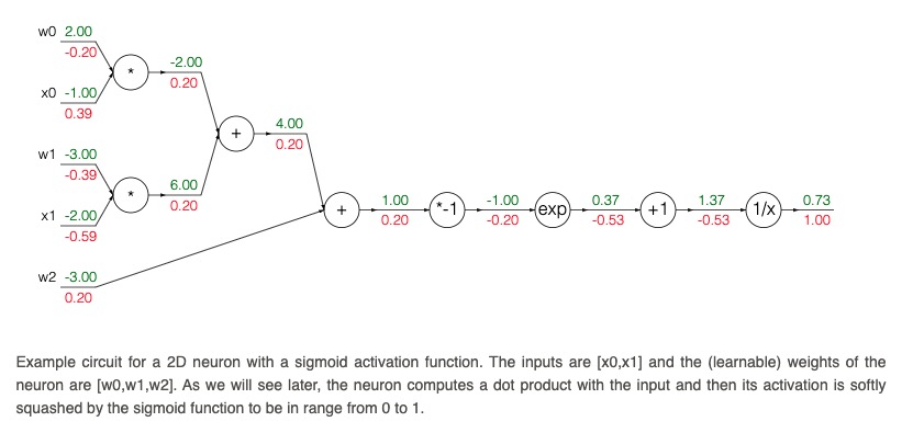 *Example of a computation graph from the excellent [CS231n](https://cs231n.github.io/optimization-2/) course*
Building a computation graph in Python Link to heading
Now we need a way to build the computation graph. How do we do this?
Let’s do it autograd style. They do it in quite a clever way.
Functions are often made up of operators from the numpy package. What they do in autograd is create a copy of the numpy package (called autograd.numpy) that behaves exactly like numpy, except it keeps track of gradients and builds a computation graph as each function is called. Then if you write import autograd.numpy as np at the top of a script, you use functions from autograd.numpy instead of functions from numpy. This is what we will build up to over the next few posts.
Let’s work with an example. Say we had the following function: $$ logistic(z) = \frac{1}{1 + \exp(-z)} $$
We would implement this in code like this
def logistic(z): return 1 / (1 + np.exp(-z))
What’s cool is numpy uses operator overloading, meaning it replaces operators like $+, \times, / $ with its own equivalents np.add, np.multiply, np.divide. It does this by defining the dunder methods __add__,__mult__,__div__ in the numpy.ndarray class. By defining these methods it means that if you pass in a ndarray to logistic(z), it will use np.add when it encounters a + sign. The effect of this is that logistic(z) gets transformed into something like this:
def logistic2(z): return np.reciprocal(np.add(1, np.exp(np.negative(z))))
Let’s see how Python breaks down this expression. Breaking an expression down has the same effect as constructing a number of intermediate variables, one for each operation, where each intermediate variable stores the result of that operation with the previous one. These operations are called primitives and they are important later.
Let’s call the intermediate variables $t_1, t_2, t_3…$, the input to the function $z$, and the final value $y$.
def logistic3(z):
    t1 = np.negative(z)
    t2 = np.exp(t1)
    t3 = np.add(1, t2)
    y = np.reciprocal(t3)
    return y
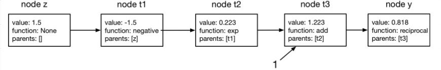
We want to turn logistic3 into a computation graph, with nodes and links between them. Here’s what this graph looks like.

We will below define a class called Node and each node in the graph will be a member of this class. Each node links together by having a parents attribute that stores the nodes pointing to it in the graph. The leaf nodes above are $1$ and $z$, and the root node is $y$. The leaf nodes are typically constants or variables passed into the function, while the root node is the scalar-valued output of the function. Leaf nodes do not have parents.
Below is a representation of the computational graph using Nodes. The numbers in value indicate the value of that intermediate variable. The function was given $z=1.5$ as an input and returns $y=0.818$.
Let’s confirm we get the same answer.
np.round(logistic3(1.5),3) # gives 0.818
Constructing the Node class, version 1 Link to heading
Now we can construct a first version of the Node class. For each Node, we need at least value, a function (fun) and parents.
We also will create a function called initialise_root that starts off the graph. A root of the tree doesn’t have any parents, its function is just the identity function, and it has no value.
class Node:
    """A node in a computation graph."""
    def __init__(self, value, fun, parents):
        self.parents = parents
        self.value = value
        self.fun = fun
Now we have the Node class, we could manually build a computational graph if we wanted to. Let’s create a Node for each intermediate variable. (We don’t create a Node for 1 or other scalars).
val_z = 1.5
z = Node(val_z, None, [])
val_t1 = np.negative(val_z)
t1 = Node(val_t1,np.negative, [z])
val_t2 = np.exp(val_t1)
t2 = Node(val_t2, np.exp, [t1])
val_t3 = np.add(val_t2, 1)
t3 = Node(val_t3, np.add, [t2])
val_y = np.reciprocal(val_t3)
y = Node(val_y, np.reciprocal, [t3])
print(round(y.value,3)) #  0.818, same answer as before
We did it! A basic computational graph is stored in y. This has links back to each intermediate Node. You can look at the parents attribute of y to traverse back through the graph. And looking at the value attribute of y, it has the same answer as just evaluating logistic3(1.5). We could use this graph for backpropagation if we wanted to.
Creating the computational graph this way, though, is both manual and clunky. In the next article we will learn how to build graphs automatically.
Again, this is the first post in a series on computational graphs. You can go to the next post or skip ahead to the third post.
Resources Link to heading
- Here are some useful lecture slides by Roger Grosse: https://www.cs.toronto.edu/~rgrosse/courses/csc321_2018/slides/lec10.pdf
- This gives some details of autodiff in PyTorch: https://towardsdatascience.com/pytorch-autograd-understanding-the-heart-of-pytorchs-magic-2686cd94ec95