Notes on DeepFool
Paper: Deepfool: a simple and accurate method to fool deep neural networks. (Moosavi-Dezfooli et al, 2016).
Idea: If you want to find an adversarial example to an image, look for the closest decision boundary, and then move the image towards a linear approximation of the decision boundary by orthogonally projecting it onto the boundary. Once it crosses the boundary it will be an adversarial image.
Background Link to heading
Affine functions. These are very similar to linear functions. The only difference is that while a linear function fixes the origin, an affine function doesn’t have to. An affine function is just a linear function that has been translated. In terms of a neural network, it’s usually the input matrix multiplied by the weight matrix. In the paper an affine classifier is defined as $f(\mathbf{x} = \mathbf{w}^T\mathbf{x} + b)$ although it can apply to anything of the form $wx + b.$
Level sets. A level set is a set where a function is equal to a constant value $c$. It is defined as $ L_c(f) = { (x_1, \cdots, x_n) : f(x_1, \cdots, x_n) =c }$. If there are two variables $x_1, x_2$, the level set is a line or curve; if there are three variables $x_1, x_2, x_3$, the level set is a plane or surface; for more variables the level set forms a hyperplane or hypersurface. The paper defines decision boundaries as level sets: i.e. $\mathscr{F} = {\mathbf{x} : \mathbf{w}^T\mathbf{x}+b = 0 }$.
Function linearisation. Say you had a function $f(x)$. The idea of linearisation is the tangent line at the point $(a, f(a)$ will approximate the function $f(x)$ well for $x$-values near $a$.
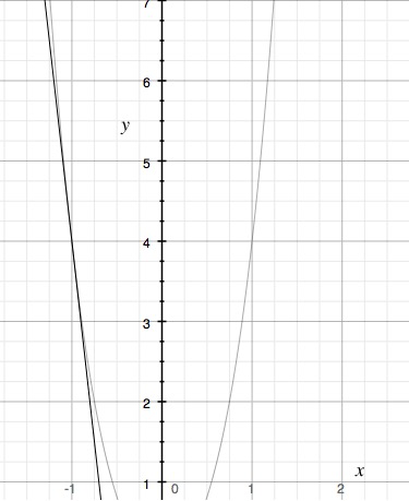
The slope of the curve at $x=-1$ is a good approximation of the curve near that point.
You can approximate the output of $f$ at a point $x$ by calculating $f(x) = f(a) + f’(a)(x-a)$, the first order Taylor expansion around the point $a$. For the curve above, $a=-1$. As you get further and further away from $a=-1$, the approximation gets worse and worse.
For example, say $f(x) = \sqrt{x}$ , and you wanted to know the value $f(x)$ at a point $x=4.001$ (i.e. $\sqrt{4.001}$ ) using a linear approximation. You would calculate $f(a) + f’(a)(x-a)$ which equals $\sqrt{a} + \frac{1}{2\sqrt{a}}(x-a)$. You might use $a=4$ as a close value. So $x = 4.001$ and $a=4$, and the linear approximation is $f(x) = \sqrt{4.001} = \sqrt{4} + \frac{(4.001 - 4)}{2\sqrt{4}} = 2.0025$.
Description Link to heading
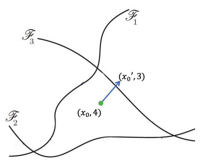
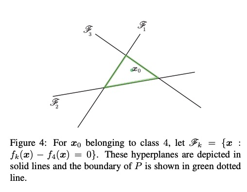
Overview: Say we are attacking $\mathbf{x}_0$, which has true label as digit 4, and we want to classify it as a 3. Then the decision boundary is given by the level set $\mathscr{F_3} = {\mathbf{x}:F(\mathbf{x})_4 - F(\mathbf{x})_3 = 0 }$.
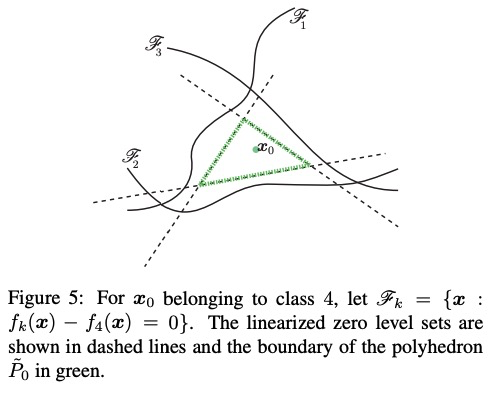
Let $f(\mathbf{x}) = F(\mathbf{x})_4 - F(\mathbf{x})_3 $. The hyperplane of the decision boundary is linearised with a first-order Taylor expansion: $\mathscr{F’_3} = {\mathbf{x}: f(\mathbf{x}) \approx f(\mathbf{x}_0) + \langle \nabla_\mathbf{x} f(\mathbf{x}_0) \cdot (\mathbf{x}-\mathbf{x}_0) \rangle = 0 }$. Then an orthogonal vector $\mathbf{r}(\mathbf{x}_0)$ is calculated from $\mathbf{x}_0$ to $\mathscr{F}’_3$, which is the same as finding $\mathbf{x}_0$ projected onto the plane $\mathscr{F}’_3$. The vector $\mathbf{r}(\mathbf{x}_0) $ is the perturbation that creates the adversarial example : it shifts $\mathbf{x}_0$ beyond the decision boundary $\mathscr{F}_3$
Hyperplanes $\mathscr{F}_i$ separate datapoints of different classes. (Adversarial Attacks and Defenses in Images, Graphs and Text: A Review., Xu et al (2019))
Details Link to heading
Start with an affine/linear classifier, $f(x) = \mathbf{w}^T\mathbf{x}+b$.
The decision boundary is the hyperplane $\mathscr{F} = {x: \mathbf{w}^T\mathbf{x}+b=0 }$.
The robustness of $f$ at a point $ x_0$ is called $\Delta(x_0;f)$ and is the shortest distance between $x_0$ and $\mathscr{F}$ : the smallest amount of perturbation required to changed the labelled class of the image. You find this distance by calculating the orthogonal projection of $\mathbf{x_0}$ onto $\mathscr{F}$ and it works out to be $\mathbf{r}_*(\mathbf{x}_0) := - \frac{f(\mathbf{x}_0)}{||\mathbf{w}||^2_2} \mathbf{w}$, a closed-form solution.
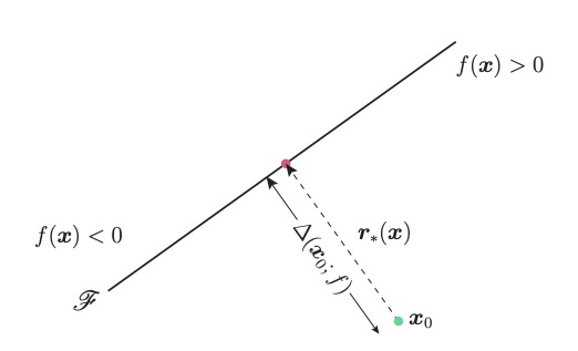
Figure 2 of the DeepFool paper.
So that’s for an affine classifier $f$.
Next comes the case where $f$ isn’t linear, but instead some curved surface. Like before, we want to find the distance $\mathbf{r}_*(\mathbf{x}_0)$, the minimal perturbation before the label of $\mathbf{x}_0$ is changed.
Now there isn’t a closed-form solution for this, so an iterative method is used.
- Start off at $\mathbf{x}_0$.
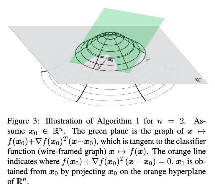
- Linearise $f$ around the point $\mathbf{x}_0$ to get a hyperplane linear approximation for $f$. Use the first order Taylor series approximation: $f_{approx} = f(\mathbf{x}_0) + \nabla f(\mathbf{x}_0)^T (\mathbf{x} - \mathbf{x}_0)$
- From the affine case, we had a closed form solution to find $\mathbf{r}_*(\mathbf{x}_0)$, the projection of $\mathbf{x}_0$ onto $\mathscr{F}$, or the minimal perturbation required to change the classification. Now we use it for our linear approximation. Add a perturbation $\mathbf{r}_0$ to $\mathbf{x}_0$, given by $\text{argmin}_{\mathbf{r}_0}||\mathbf{r}_0||_2 \text{ subject to }f(\mathbf{x}_0) + \nabla f(\mathbf{x}_0)^T \mathbf{r}_0 =0 $. This is the minimum perturbation needed to get to the linear approximation of the decision boundary. This gives you a new point $\mathbf{x}_1 = \mathbf{x}_0 + \mathbf{r}_0 $
- Have we changed classification yet? If we have, stop. If we haven’t, it’s time for the next iteration.
- Calculate a new $f_{approx}$, the linear approximation to $f$ using the point $\mathbf{x}_1$. Work out where $f_{approx} =0$ and orthogonally project $\mathbf{x}_1$ onto this line (this gives you $\mathbf{x}_2$). Check the classification: if it has changed, stop, else keep going.
Visualisation of the method, with original caption
This has all been for the binary case. I won’t go into detail for the multi-class case, but the same ideas hold, except you have multiple decision boundaries.
The multiclass affine case
You are trying to move a point towards (and eventually over) the nearest decision boundary, since that is the one with the least perturbation.
If you have a curved decision boundary, you’ll need to take linear approximations and do the iterative algorithm again.
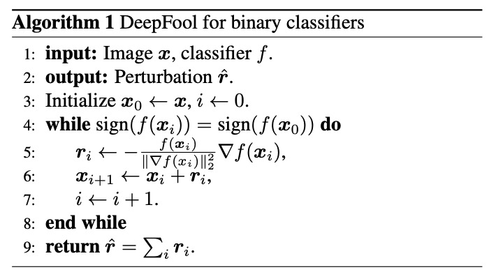
Here is the pseudocode for this algorithm:
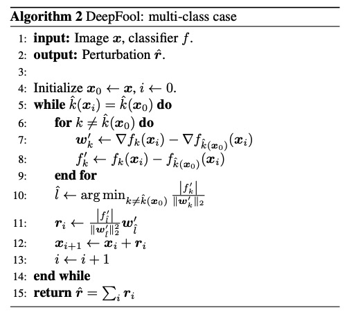
The method is a bit slower than FGSM, but it works much better. It’s been superceded by other methods today.