Data Valuation using Reinforcement Learning (dvrl)
Data Valuation using Reinforcement Learning Link to heading
Paper link: https://arxiv.org/pdf/1909.11671.pdf
At a glance Link to heading
Machine learning models use data for training. But not all data points are equally valuable.
A data point can be low-quality for a variety of reasons, such as incorrect labelling, noisy input, being too common, or it’s not from the same distribution as the test set. Whatever the case, removing bad datapoints tends to increase model performance. But how do you know which datapoints are valuable and which aren’t? That is the domain of data valuation.
The data valuation problem has been tackled before with techniques like leave-one-out model evaluation or Shapley values. These techniques have their flaws. This paper demonstrates a new algorithm called DVRL that performs better than these other techniques. It also scales much better with dataset size.
DVRL requires a dataset and an predictive model. For example, the CIFAR-10 dataset and a predictive classification model. The goal of DVRL is to give a score to each row of the dataset that’s based on its contribution to model predictive accuracy.
This score is a measure of the quality of the data point. Critical data points are given a high score, and low-quality data points are given a low score.
Overview Link to heading
The algorithm is comprised of two smaller models.
A model to give a score for each training data point. The score can be translated into the probability of using that training datapoint in the second model. Higher scores mean the data is more useful. This model is called the data value estimator.
A model to assess predictive model performance. It takes as input a selection of rows of the dataset, which are chosen by the first model. Model performance is assessed using a separate validation dataset. This model is called the predictor.
Here’s a diagram of the whole process. The data value estimator is in blue. The predictor is in red.
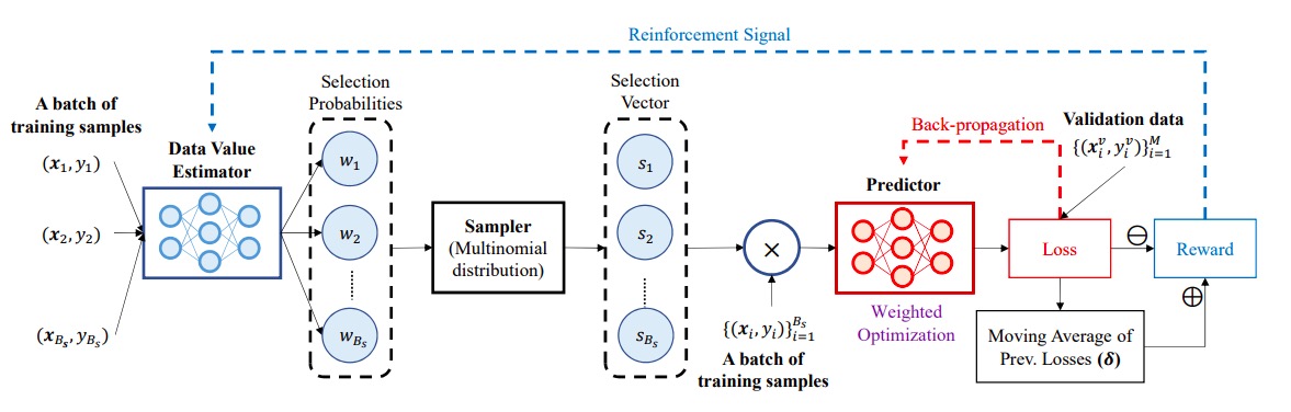
The two models work together. The output of the data value estimator determines the input of the predictor model. The output of the predictor model is used to update the weights of the scoring model.
And so on.
Data value estimator Link to heading
DVRL uses a policy gradient algorithm called REINFORCE to update the weights of the data value estimator model. This algorithm requires a reward, which comes from the performance of the predictor model on a validation set. This is measured in something like cross-entropy or MSE or L1 loss and so forth.
For each subset of rows, its performance is compared against a moving average of the last N runs. Did it do well compared to the last runs? High reward. Not so well? Low reward. REINFORCE then updates the weights of the data value estimator model, incentivising it to try and produce selections of rows that give high performance. Eventually the weights will hit convergence and the algorithm is finished.
How are the data points selected? The data value estimator model will output a probability between 0 and 1 for each row, which is its chance to be selected. Then each row is sampled using that chance. It’s like you’re flipping a coin, where heads the row is selected, and tails it isn’t, except that the chance for getting a head is different for every row.
Predictor models Link to heading
Let’s talk a bit about the predictor model. This model has to be trained as well. How do you do that?
Firstly, there’s nothing that says you can’t use a pre-trained model. So you could start it off with that. But you’d still want to train the model a bit.
It turns out that you can use mini-batch updating here. Start off with the selection of rows chosen by the data value estimator model. Then sample a mini-batch from this and use it to update the predictor model weights. Repeat this a given number of times to train the model.
How many rows do you need for the validation set? Like all things machine learning, more is usually better. But you can get away with surprisingly few rows. 400 is a good amount, but even 10 will give reasonable performance.
Training time Link to heading
Finally, what determines the model training time? It’s not proportional to the size of the dataset, which is a major advantage over other methods. Rather, it depends on parameters like how many mini-batch updates you do, or how long it takes the data value estimator model to converge.
Here’s how the process works on a real dataset like CIFAR-10. First, a baseline model is trained using the entire dataset. This model becomes the predictor model. Next the algorithm above begins, fine-tuning the weights of both models until convergence. The total time is roughly twice that needed of just the baseline model. So DVRL takes twice as long as regular training.
Use cases Link to heading
DVRL performs well. It’s better than the existing approaches, and it’s also quite a bit quicker. So that’s good.
What can you use it for? Here are some use cases for DVRL mentioned in the paper.
- Identifying high value datapoints. These are the ones that your model learns the most from. You can use this for some insights; these points are represented well in the validation set.
- Removing low value datapoints. Your model does better without them.
- Discovering corrupted samples. DVRL can identify mislabelled data by giving it a low score. You can use this to remove the offending points from your dataset.
- Robust learning. Instead of removing low-value datapoints, we keep them in, but use DVRL to reduce their impact on the final model. Performance is typically better than if you just removed them.
- Domain adaptation. Your training set is from one distribution, but your validation and test sets are from a different one. DVRL selects those points from the training set that are most like the test set; in other words, those points that best match the test set distribution.