Measuring the Intrinsic Dimension of Objective Landscapes (2018) - summary
The paper in one sentence. The Pareto principle for neural networks: what’s the least number of parameters needed for to achieve most of the results?
Structure of this article. I give an introduction to objective landscapes and talk about how to define solutions. I use these concepts to describe the subspace training method. Finally, I summarise the key results of the paper.
Objective landscapes Link to heading
For every combination of neural network architecture and dataset, the shape of the objective/loss function is fixed. We call this shape the objective landscape and it has many dimensions: one for each parameter in the network.
You can imagine the objective landscape for the two-parameter case as hills and valleys of a landscape. It’s a bit harder for three dimensions, but I like to imagine it as a LED light cube, where every point has a different colour, and darker points represent lower values.
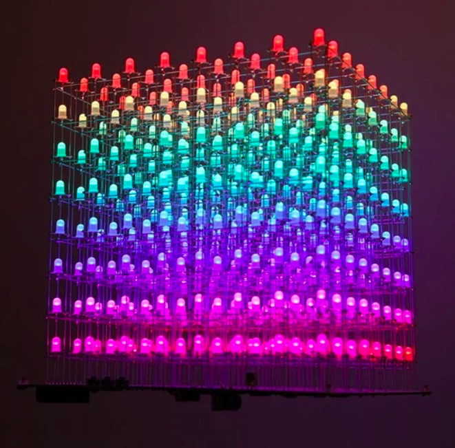
The objective landscape is more continuous than this, but you get the idea.
Training a neural network means attempting to find the combination of parameters that minimises the objective landscape. For the 2D case with hills and valleys, this means the lowest point. For the 3D light cube, it’s the darkest point. Generally speaking, it’s wherever minimises the loss function.
To find the lowest point the neural network uses gradient descent. This is a stepwise procedure finding $dL/d\theta$ , the gradient of the objective function with respect to each parameter. Parameters are updated using this gradient. The overall effect is taking a step in the most “downhill” direction from the current point. Eventually you reach somewhere where you can’t go any lower and typically this is the lowest point in the landscape.
But not always. You could get stuck in a local optima: a point where you can’t go down any further, but it isn’t the lowest point of the landscape.
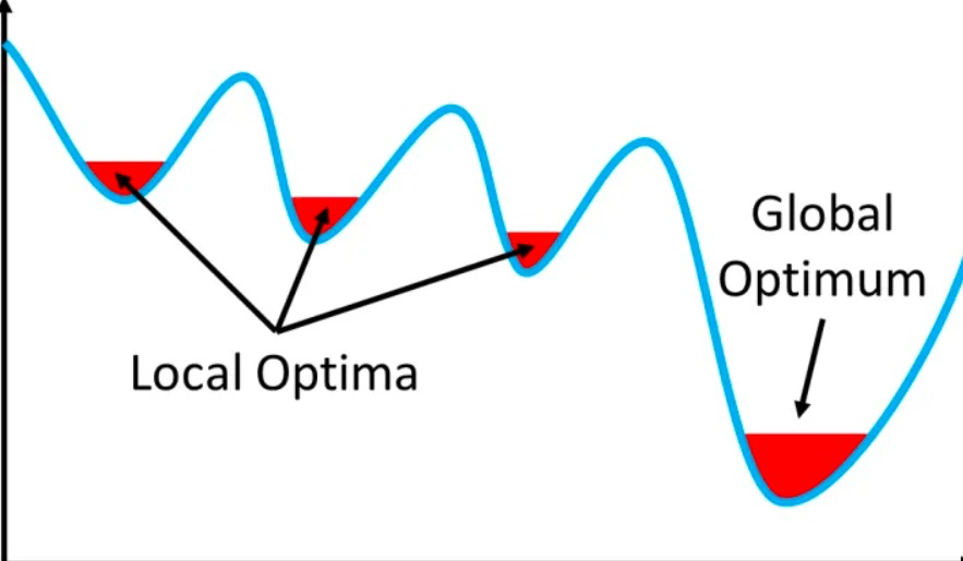
How do you know you’re at a local optima if you can’t see the entire landscape?
For higher dimensions, a bigger problem is saddle points. These are areas where the landscape is flat in many dimensions, perhaps because there are many redundant parameters with little effect on the objective function. Saddle points are problematic: many optimisers have trouble escaping them and it’s easy to be stuck in these areas for a long time. Removing redundant parameters in a neural network can reduce chances of encountering saddle points.
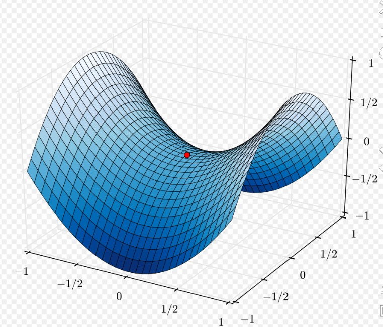
A saddle point in the x-y plane
That’s not the only reason to reduce network parameters. Neural networks take up a lot of space. If you make networks smaller, they can be used more widely: IoT devices, webpages, mobile phones.
Solutions Link to heading
We usually talk about minimising the loss function. But it’s hard talking about loss all the time. You can’t compare loss between datasets, and loss is hard to interpret without any context. It’s easier to use something like validation accuracy or reward instead. For simplicity, anytime I talk about performance, I’m talking about validation accuracy.
For many datasets we know the best performance achieved to date. For example, the current best performance on MNIST is 99.79%. Of course, for many more datasets we don’t know the best performance, but for now let’s assume we know it.
Let’s call the model with the best performance the baseline model, its performance the baseline performance, the point on the objective landscape corresponding to its parameters the 100% solution, and its number of parameters $d_{int100}$. You might have a few models with statistically indistinguishable solutions around the 100% mark, and in that case you can consider them all 100% solutions.
It turns out achieving a 100% solution is hard, and you can’t remove many parameters if you are insistent on 100% performance. It’s much easier to get a 90% solution: a solution achieving 90% baseline performance. All points achieving at least 90% baseline performance on a task are called 90% solutions. The number of parameters used in a 90% solution is called $d_{int90}$ and this number is often much lower than $d_{int100}$.
Here’s a heuristic to classify all points on the objective landscape as solutions or non-solutions. A point achieving at least 90%1 baseline performance is a solution. The set of all solutions is called the solution set2.
Subspace training Link to heading
To recap, typically we want to find the lowest point in the $D$-dimensional objective landscape, where $D$ is the number of parameters in the neural network. Let’s store the $D$ parameters in a vector and call it $\theta^{(D)}$.
We want to reduce the number of parameters. We know many are redundant, not required, or used only to make training faster. It’s very likely that we don’t require all parameters to find a solution. So what if we only used some smaller number $d$ parameters, instead of $D$?
Now we come to the essence of the paper: what’s the least number of parameters we could use, and still reliably find a solution? This number of parameters is called the intrinsic dimension and is denoted $d_{int}$.
Let’s say your neural network has $D=3$ parameters, and you think you can find a solution using $d=2$ parameters. If this is true you could draw a random plane through $\mathbb{R}^3$ so the plane and the solution set intersect.
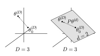
Figure 1 from the paper. On the left we have optimisation in the original, three dimensional space. On the right we create a plane (or subspace) and constrain our parameters to the plane. The plane lies in the three dimensional $\mathbb{R}^3$, but the surface of the plane is in $\mathbb{R}^2$.
Okay. How do we do this?
First, define the plane in $\mathbb{R}^2$. There are two parameters, so let’s call these parameters $\theta^{(2)}$ and start them off at zero. These parameters are different from any parameters in the original $\mathbb{R}^3$ space.
You can’t optimise directly in $\mathbb{R}^2$ since the neural network requires a vector in $\mathbb{R}^3$. You need a way to map from the $\mathbb{R}^2$ subspace to the $\mathbb{R}^3$ space. This is a linear mapping, so we can use a matrix with shape $3 \times 2$. Call this matrix $P$ 3. Then $P \theta^{(2)}$ maps from $\mathbb{R}^2 \to \mathbb{R}^3$.
There’s a few ways to initialise $P$, but let’s make it a dense matrix for now, with unit length columns.4 $P$ has some interesting properties. If $P$ is orthonormal (i.e. orthogonal and unit length basis vectors), then you have a one-to-one distance mapping between $\mathbb{R}^2$ and $\mathbb{R}^3$. In other words, if you take a step with length one unit in $\mathbb{R}^2$, you’ll move one unit in $\mathbb{R}^3$.
Next, you need a starting point in $\mathbb{R}^3$. Call this $\theta_0^{(3)}$ and randomly initialise it.
Now we define the equation to update $\theta^{(3)}$:
$$ \theta^{(3)} = \theta_0^{(3)} + P\theta^{(2)}$$
(or more generally)
$$ \theta^{(D)} = \theta_0^{(D)} + P \theta^{(d)} $$
Training in a subspace has a few differences to the usual full-dimensional way.
-
Start off with $\theta^{(2)}$ equal to zeros. (This means that the first value of $\theta^{(3)}$ is the randomly initialised $\theta^{(3)}_0$.)
-
Perform the feed-forward step using $\theta^{(3)}$ and calculate the loss function $L$.
-
Perform backpropagation to find $dL/d\theta^{(2)}$. Usually backpropagation stops after finding $dL/d\theta^{(3)}$, but since $\theta^{(3)}$ is defined in terms of $\theta^{(2)}$ the autodiff algorithm will continue and find $dL/d\theta^{(2)}$.
-
Use the gradient $dL/d\theta^{(2)}$ to take a step in the $\mathbb{R}^2$ space that most minimises the loss function.
-
Convert the step in $\mathbb{R}^2$ to a step in $\mathbb{R}^3$ through $P\theta^{(2)}$ and update $\theta^{(3)}$ with $ \theta^{(3)} = \theta_0^{(3)} + P\theta^{(2)}$
-
Perform feed-forward step using the new value of $\theta^{(3)}$ and calculate the loss function $L$
etc.
Can you find a solution? If you can, then $d_{int}$, the intrinsic dimensionality of this network architecture on this dataset, is at least 2.
We say that $d_{int}$ is the lowest value of $d$ for which you can find a solution. So if you found a solution by setting $d=1$, then $d_{int}$ would equal 1.
Now you see the procedure. Take a dataset (e.g. MNIST) and an architecture (e.g. LeNet). Start with $d=1$ and try to find a solution. If you can’t, try $d=2$, then $d=3$, and so on until you find the lowest value of $d$ with a solution. That value is the intrinsic dimensionality.
Results Link to heading
There’s a lot of interesting things that come out of the paper. Here is what stood out to me.
$d_{int}$ is fairly constant across network architectures for a family of models. For example, a wide range of fully-connected (FC) networks had similar values for $d_{int}$ on MNIST 5. This implies that larger networks are effectively wasting parameters.
There are significant compression benefits. To describe a network after subspace compression you need: the random seed to generate $\theta_0^{(D)}$, the random seed to generate $P$, and the $d_{int}$ parameters in the (optimised) $\theta^{(d)}$ vector. That’s not much. There’s uses here for anything with bandwidth or space concerns, like webpages and apps, or IoT devices. .
$d_{int}$ acts as an upper bound for minimum description length of a solution. If you can compress the data using (effectively) $d_{int}$ parameters, then the minimum description length (MDL) isn’t going to be higher than that.
$d_{int}$ can be used to compare architectures. Many architectures might have the same performance for a task, like a CNN and a FC network on MNIST. But the CNN is probably much more efficient than the FC network. If $d_{int}$ for the CNN is much lower than $d_{int}$ for the FC network, its MDL is probably lower, and it follows from Hinton and Van Camp (1993) that the best model is the one with the lowest MDL.
You can find $d_{int}$ for reinforcement learning tasks, too. Any task using a neural network is fair game.
Shuffling pixels increases $d_{int}$ for CNNs but not for FC models. This makes sense: convolutional layers rely on local structure in the image, while FC networks treat each pixel as independent of others around it.
Memorisation effects. Randomise the labels for training examples. The more labels are memorised by the network, the more efficient it is at memorising new, random labels. The network gets better at memorising the more data it has.
-
90%, like most whole numbers, is somewhat arbitrary but a good starting point. The authors chose 90% by looking at a few different curves of $d_{int}$ vs baseline performance and then picking a value that corresponding to where the curves started to flatten out. ↩︎
-
There’s no guarantee that the manifold of the solution set is a hyperplane or anything similarly well behaved. ↩︎
-
The paper calls $P$ a projection matrix, but it looks like $P$ is a bit different to the one described in Wikipedia. For starters, it’s not square, meaning it isn’t idempotent. ↩︎
-
The paper goes through some of the ways. You can make $P$ a dense matrix, making sure each column is orthonormal to the others. Another way is to rely on the approximate orthogonality of high dimensions to not worry about ensuring each basis vector of P is orthogonal. You can also make P a sparse projection matrix, which saves on memory and computation speed, or use the Fastfood transform to make space complexity not depend on $d$. Both of these methods are useful for higher dimensional networks. ↩︎
-
$d_{int}$ varied by a factor of around 1.33, perhaps because of noise. ↩︎