The Keras functional API: five simple examples
Building models in Keras is straightforward and easy. If you’re reading this, you’re likely familiar with the Sequential model and stacking layers together to form simple models. But what if you want to do something more complicated?
Enter the functional API. For complex models the functional API is really the only way to go - it can do all sorts of things that just aren’t possible with the Sequential model. Models with multiple inputs and outputs, models with shared layers - once you start designing architectures that need these things, you will have to use the functional API to build your model.
But using the functional API is tricky - at least, I found it tricky. What I found helpful was sitting down and coding up some examples using the Functional API - just simple examples, but enough to get going.
In this post we’ll run through five of these examples. To understand this post there’s an assumed background of some exposure to Keras and ideally some prior exposure to the functional API already. There are better resources than this in describing the basics of the functional API - below will just be examples.
Creating some sample data Link to heading
First we’ll need to set up some data to use for our examples. We’ll use numpy to help us with this. Normally I like to use pandas for these kind of tasks, but it turns out that pandas DataFrames don’t integrate well with Keras and you get some strange errors.
We’ll create two datasets: a training dataset, and a test dataset. Normally we’d create a cross validation set as well but for example purposes it’s okay to just have a test set.
The toy data will have three predictor variables ($x_1$, $x_2$ and $x_3$) and two response variables ($y_{classifier}$ and $y_{cts}$), where cts stands for continuous. We want two response variables because we’ll be building a number of models, some that predict discrete outcomes (like logistic regression) and some that predict continuous outcomes (like linear regression).
For our classifier variable $y_{classifier}$, we’ll set it equal to 1 when $ x_1 + x_2 + \frac{x_3}{3} + \epsilon > 1$, where $\epsilon \sim N(0,1)$, and $y_{classifier} = 0$ elsewhere.
For our continuous variable $y_{cts}$, we’ll set $y_{cts} = x_1 + x_2 + \frac{x_3}{3} + \epsilon $. This way both variables will look similar, and in the end we’ll have some data that isn’t linearly seperable, but good enough to train models on.
import numpy as np

n_row = 1000
x1 = np.random.randn(n_row)
x2 = np.random.randn(n_row)
x3 = np.random.randn(n_row)
y_classifier = np.array([1 if (x1[i] + x2[i] + (x3[i])/3 + np.random.randn(1) > 1) else 0 for i in range(n_row)])
y_cts = x1 + x2 + x3/3 + np.random.randn(n_row)
dat = np.array([x1, x2, x3]).transpose()
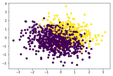
Let’s take a quick look at our data. Here’s the first two dimensions plotted with the colour symbolising different values of $y_{classifier}$:
# Take a look at the data
import matplotlib.pyplot as plt
%matplotlib inline
plt.scatter(dat[:,0],dat[:,1], c=y_classifier)
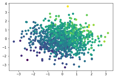
Here’s the same graph for $y_{cts}$
plt.scatter(dat[:,0],dat[:,1], c=y_cts)
Last thing we’re going to do is split up our data into a training and test set so that we can check model performance as we train it:
# Generate indexes of test and train
idx_list = np.linspace(0,999,num=1000)
idx_test = np.random.choice(n_row, size = 200, replace=False)
idx_train = np.delete(idx_list, idx_test).astype('int')

# Split data into test and train
dat_train = dat[idx_train,:]
dat_test = dat[idx_test,:]
y_classifier_train = y_classifier[idx_train]
y_classifier_test = y_classifier[idx_test]
y_cts_train = y_cts[idx_train]
y_cts_test = y_cts[idx_test]
Our data is ready - let’s train some Keras models.
# setup
from keras.models import Input, Model
from keras.layers import Dense
Example 1 - Logistic Regression Link to heading
Our first example is building logistic regression using the Keras functional model. It’s quite easy and straightforward once you know some key frustration points:
- The input layer needs to have shape
(p,)wherepis the number of columns in your training matrix. In our case we have three columns ($x_1, x_2, x_3$) so we set the shape to $(3,)$ - The output layer needs to have the same number of dimensions as the number of neurons in the dense layer. In our case we’re predicting a binary vector (0 or 1), which has 1 dimension, so our dense layer needs to have one neuron.
# Build the model with Functional API
inputs = Input(shape=(3,))
output = Dense(1, activation='sigmoid')(inputs)
logistic_model = Model(inputs, output)

# Compile the model
logistic_model.compile(optimizer='sgd',
                       loss = 'binary_crossentropy',
                       metrics=['accuracy'])

# Fit on training data
logistic_model.optimizer.lr = 0.001
logistic_model.fit(x=dat_train, y=y_classifier_train, epochs = 5,
                   validation_data = (dat_test, y_classifier_test))
We’ll use our trick from before to see the rough figure for what this eventually converges to:
logistic_model.fit(x=dat_train, y=y_classifier_train, epochs = 500, verbose=0,
                   validation_data = (dat_test, y_classifier_test))
logistic_model.fit(x=dat_train, y=y_classifier_train, epochs = 1, verbose=1,
                   validation_data = (dat_test, y_classifier_test))
Train on 800 samples, validate on 200 samples
    Epoch 1/1
    800/800 [==============================] - 0s - loss: 0.3300 - acc: 0.8562 -
                                              val_loss: 0.3244 - val_acc: 0.8450
If we look at our weights we can see that our logistic model has roughly the right idea about what they should be:
# true weights: 1,1,1/3
logistic_model.get_weights()
# gives [ 1.36166012],[ 1.38322246],[ 0.55906934]]
It’s a bit much to expect perfect performance given the amount of noise in the data. This is a pretty good result.
Example 2 - Linear Regression Link to heading
Here we’ll construct a basic linear regression with $y_{cts}$ as the dependent variable and $x_1$, $x_2$ and $x_3$ as the predictor variables (remember which are stored inside the numpy array dat. You’ll see that the code for linear regression looks a lot like that for logistic regression above - we just use a linear activation function instead of a sigmoid one.
inputs = Input(shape=(3,))
output = Dense(1, activation='linear')(inputs)
linear_model = Model(inputs, output)

linear_model.compile(optimizer='sgd', loss='mse')

linear_model.fit(x=dat_test, y=y_cts_test, epochs=50, verbose=0)
linear_model.fit(x=dat_test, y=y_cts_test, epochs=1, verbose=1)
One way to see if our model is a good fit or not is by looking at some of the errors and seeing if there is a pattern.
preds = linear_model.predict(dat_test)
plt.scatter(x=dat_test[:,0], y= np.array(preds) - np.array(y_cts_test).reshape(200,1))
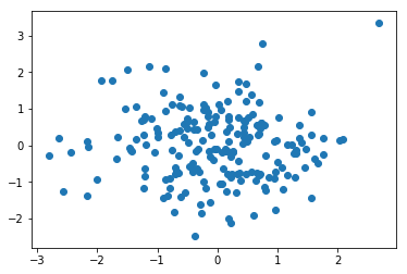
Doesn’t look like it to me!
Example 3 - Simple Neural Network Link to heading
Below is how to implement a simple neural network with one hidden layer. Again, it’s pretty straightforward.
inputs = Input(shape=(3,))
x = Dense(50, activation='relu')(inputs)
output = Dense(1, activation = 'sigmoid')(x)
n_net = Model(inputs, output )

n_net.compile(optimizer='adam', loss='binary_crossentropy', metrics=['accuracy'])

n_net.fit(x=dat_train, y=y_classifier_train, epochs=10,
verbose=1, validation_data=(dat_test, y_classifier_test))
We get up to about 84% accuracy on the test set with this model.
Example 4 - Deep Neural Network Link to heading
Below we train a neural network with a large number of hidden layers. We also add Dropout to the layers to reduce overfitting.
It can be useful sometimes to use for loops and if statements when using the Functional API, particularly for complicated models.
from keras.layers import Dropout
# specify how many hidden layers to add (min 1)
n_layers = 5

inputs = Input(shape=(3,))
x = Dense(200, activation='relu')(inputs)
x = Dropout(0.4)(x)
for layer in range(n_layers - 1):
x = Dense(200, activation='relu')(x)
x = Dropout(0.3)(x)
output = Dense(1, activation='sigmoid')(x)
deep_n_net = Model(inputs, output)

deep_n_net.compile(optimizer = 'adam', loss= 'binary_crossentropy', metrics=['accuracy'])

deep_n_net.fit(dat_train, y_classifier_train, epochs = 50, verbose=0,
validation_data = (dat_test, y_classifier_test))
deep_n_net.fit(dat_train, y_classifier_train, epochs = 1, verbose=1,
validation_data = (dat_test, y_classifier_test))
This model does about as well as the previous neural network. It could probably do better by tuning the hyperparameters, like the amount of dropout or the number of neural network layers.
Example 5 - Simple Neural Network + Metadata Link to heading
One use case for the Functional API is where you have multiple data sources that you want to pull together into one model.
For example, if your task is image classification you could use the Sequential model to build a convolutional neural network that would run over the images. If you decide to use the Functional API instead of the Sequential model, you can also include metadata of your image into your model: perhaps its size, date created, or its tagged location.
We’ll demonstrate this technique of combining multiple data sources by creating two vectors of “metadata” for use with our contrived dataset. It would be nice if they were helpful, so we’ll ‘cheat’ and make them equal to y_classifier plus some random noise. The metadata will help illustrate incorporating multiple sources of information in one model.
Our model architecture below will have two hidden layers with the metadata added after the first of them.
metadata_1 = y_classifier + np.random.gumbel(scale = 0.6, size = n_row)
metadata_2 = y_classifier - np.random.laplace(scale = 0.5, size = n_row)
metadata = np.array([metadata_1,metadata_2]).T

# Create training and test set
metadata_train = metadata[idx_train,:]
metadata_test = metadata[idx_test,:]
We’ll need the concatenate layer to merge the two data sources together.
from keras.layers import concatenate
Let’s build the model now. Note how we have two input layers: one for the original data and one for the metadata. Both sets of data go through a dense layer and a dropout layer. They are then combined with the concatenate layer, go through another dense and dropout layer before a final dense layer gives the output values.
input_dat = Input(shape=(3,)) # for the three columns of dat_train
n_net_layer = Dense(50, activation='relu') # first dense layer
x1 = n_net_layer(input_dat)
x1 = Dropout(0.5)(x1)

input_metadata = Input(shape=(2,))
x2 = Dense(25, activation= 'relu')(input_metadata)
x2 = Dropout(0.3)(x2)

con = concatenate(inputs = [x1,x2] ) # merge in metadata
x3 = Dense(50)(con)
x3 = Dropout(0.3)(x3)
output = Dense(1, activation='sigmoid')(x3)
meta_n_net = Model(inputs=[input_dat, input_metadata], outputs=output)

meta_n_net.compile(optimizer='sgd', loss='binary_crossentropy', metrics=['accuracy'])
When fitting this model remember to supply two sets of data, not just one.
meta_n_net.fit(x=[dat_train, metadata_train], y=y_classifier_train, epochs=50, verbose=0,
validation_data=([dat_test, metadata_test], y_classifier_test))
meta_n_net.fit(x=[dat_train, metadata_train], y=y_classifier_train, epochs=1, verbose=1,
validation_data=([dat_test, metadata_test], y_classifier_test))
This model gives 95% accuracy on the test set! It’s clear that adding information here from another source helped our model to make good predictions.
Summary Link to heading
At this point you should hopefully know enough about the functional API to be able to start to decipher the complicated models that exist out there. The functional API can also do much more than what is described in this post.