Exploring policy evaluation in reinforcement learning
Today, we explore policy evaluation. We’ll explain it by example.
Given a policy, policy evaluation aims to find the value of each state $ v_\pi (s) $. That’s what we’ll be doing with the equiprobable random policy.
The scenario Link to heading
Taken from the textbook “An Introduction to Reinforcement Learning” (Sutton and Barto), Gridworld is the following scenario.
There is a grid with sixteen squares. The top left and the bottom right square are terminal squares. The goal of the agent is to reach those squares, and it is penalised -1 for every transition until it does so.
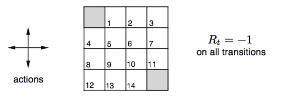
An Introduction to Reinforcement Learning’ - Sutton and Barto. Example 4.1
The agent can move left, up, down or right; not diagonal. If the agent tries to move off the grid (like moving left at the square 8, or down at the square 14) it just stays where it is, but still is penalised -1.
The approach Link to heading
The Gridworld is small enough for us to find the value of each state directly - that is, go through all states sequentially and calculate their value function $v_\pi (s)$. There is a dependence on $\pi$ in the value function, meaning the values we find will be different if we use a different policy.
Once we have $v_\pi (s)$ we can also find the action value function $ q_\pi (s,a) $. This isn’t the only method to find $ q_\pi (s,a) $ - it can also be found as $v_\pi (s)$ is found, but here we’ll do it afterwards.
The setup Link to heading
We’ll use Python to model this. The code below
- defines the size of the grid (
nrowandncol) - initialises our value function $v_\pi (s)$ as a matrix of zeros
- creates the grid, with empty strings for squares and “T” as the terminal states
- defines the action the agent can take: up, down, left and right. Moving in a direction is represented by the resulting coordinate difference. For example, moving down one square would change the agent’s coordinate by one row, or a coordinate difference of (1,0).
- creates the policy, which for this example are the probabilities of moving up, down, left and right. We follow an equiprobable policy, meaning we choose one of the four directions at random.
## Import packages and set initial variables
import numpy as np
np.random.seed = 123
nrow = 4
ncol = 4


# This is our value function
v = np.zeros((nrow,ncol))

## Create the grid
# The grid will be made up of empty strings except for the terminal states,
# which will have 'T'
grid = np.zeros((nrow,ncol), dtype='str')
grid[0,0] = 'T'
grid[nrow-1,ncol-1] = 'T'

# Set up the coordinate changes of moving up, down, left, right
# Note: this is the oppposite of the xy-plane. Rows is the x-axis,
# columns is the y-axis
actions = [(-1,0), (1,0), (0,-1), (0,1)]
# The cutoffs represent an equiprobable random policy
# We select a random number later and the cutoffs are the ranges for
# each action.
cutoffs = np.array([0.25, 0.5, 0.75, 1])
Finding the value function Link to heading
Once the grid is created we can calculate the value function for each state. We’ll find it by simulating n episodes for each starting point on the grid, and taking the average return across episodes.
Each episode runs for a maximum of k time steps. The episodes won’t run for exactly k steps because sometimes the agent will hit the terminal state.
The value function depends on k . A higher k will give the agent more time to find the terminal states, and also that the agent will accumulate more (negative) rewards.
## Calculating the value function by simulation
n = 2000  # Number of episodes
k = 10   # Maximum number of time steps per episode
for x in range(nrow):
    for y in range(ncol):
        G = np.zeros(n)  # Our return for each episode
        for i in range(n):
            coord = [x,y]  # Starting position of the agent
            r=0; cnt=0  # Reset from last simulation
            while grid[tuple(coord)] != 'T' and cnt < k:
                # get next coordinate
                rnum = np.random.uniform()
                coord = np.add(coord, actions[np.min(np.where(rnum < cutoffs))])
                # adjust for going off the grid
                coord[0] = max(0, coord[0]); coord[0] = min(coord[0], (nrow-1))
                coord[1] = max(0, coord[1]); coord[1] = min(coord[1], (ncol-1))
                # allocate reward, increase counter
                r += -1; cnt += 1
            G[i] = r
        # The value is the average return for that starting state.
        v[x,y] = np.mean(G)
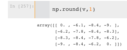
For n = 2000 and k = 10 we get as our value function
which is almost identical to the k = 10 value function given by Sutton and Barto
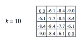
meaning we’ve done a good job!
Finding the action-value function Link to heading
One way to find the action-value function $q_\pi (s,a)$ is to wait until you have found the value function $v_\pi (s)$ and then use the relationship:
$$ q_\pi (s, a) = \sum_{s’} p(s’ | s,a) \left[ r(s,a,s’) + \gamma v_\pi(s’) \right] $$
There is no uncertainty in Gridworld over where the agent moves once it chooses an action, so we have $ p(s’|s,a) = 1$ in all cases. The parameter $ \gamma $ is called the discount rate and is a parameter we can tweak.
Like the value function, the action-value function depends on k. The code below finds the action value function for the n = 2000, k = 10 value function $v_\pi (s)$ found earlier.
## Find the action-value function q

# Set up 3D array for q
# The first dimesnion holds the direction chosen.
# Order is up, down, left, right
q = np.zeros((4, nrow, ncol))
gamma = 0.9  # discount rate parameter
for x in range(nrow):
    for y in range(ncol):
        for i, action in enumerate(actions):
            # Get coordinate of the next state s'
            s_prime = np.add((x,y), action)
            # Adjust for going off the grid
            s_prime[0] = max(0, s_prime[0]);a s_prime[0] = min(s_prime[0], (nrow-1))
            s_prime[1] = max(0, s_prime[1]); s_prime[1] = min(s_prime[1], (ncol-1))
            # Allocate the action-value function
            q[i,x,y] = -1 +  gamma * v[tuple(s_prime)]
This gives as $q_\pi (s,a)$
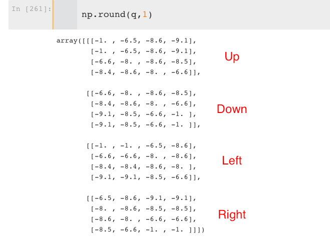
Top left and bottom right are the terminal states. The $a$’s for $q_\pi (s,a)$ are labelled red.
Intuitively these results make sense. States far away from the terminal states have a low value function and are worse for the agent. Standing next to the terminal state is good, particularly if your next action brings the agent to the terminal state.
What does this mean? Link to heading
The random policy is terrible. The agent is pulled in directions that don’t make sense; into walls, away from the terminal state around in circles. It finds the terminal state by luck, nothing more.
Maybe it would make sense to update the policy as we go…