A simple CNN with Pytorch
Find the code for this blog post here: https://github.com/puzzler10/simple_pytorch_cnn
We will build a classifier on CIFAR10 to predict the class of each image, using PyTorch along the way.
This is basically following along with the official Pytorch tutorial except I add rough notes to explain things as I go. There were a lot of things I didn’t find straightforward, so hopefully this piece can help someone else out there. If you’re reading this, I recommend having both this article and the Pytorch tutorial open.
Start off with initialisations
import torch
import torchvision
import torchvision.transforms as transforms
import numpy as np
import matplotlib.pyplot as plt
import pandas as pd
%matplotlib inline
path_data = './data/'
Getting the data Link to heading
Pytorch provides a package called torchvision that is a useful utility for getting common datasets. Using this package we can download train and test sets CIFAR10 easily and save it to a folder. The training set is about 270MB. If you’ve already downloaded it once, you don’t have to redownload it.
train = torchvision.datasets.CIFAR10(root=path_data, train=True, download=True)
test = torchvision.datasets.CIFAR10(root=path_data, train=False, download=True)
Files already downloaded and verified
Files already downloaded and verified
Let’s look at train. What we get from this is a class called CIFAR10.
type(train)
torchvision.datasets.cifar.CIFAR10
Let’s inspect this object. There’s a few useful things you can do with this class:
train.classes: view the output classes as stringstrain.targets: numericalised output classes (0-9)train.class_to_idx: mapping betweentrain.classesandtrain.targetstrain.data: has the raw data as a PIL Image, held innumpy.ndarrayformat in the range [0,255], in the order (H x W x C). This has shape(50000, 32, 32, 3).
As always train.__dict__ lets you see everything at once.
Now its time to transform the data. Use torchvision.transforms for this. Some basic transforms:
-
transforms.ToTensor(): convers PIL/Numpy to Tensor format. It converts a PIL Image or numpy.ndarray with range [0,255] and shape (H x W x C) to a torch.FloatTensor of shape (C x H x W) and range [0.0, 1.0]. So this operation also rescales your data. It’s not a simple “ndarray –> tensor” operation. -
transforms.Normalize(): normalises each channel of the input Tensor. The formula is this:input[channel] = (input[channel] - mean[channel]) / std[channel]. You have to pass in two parameters: a sequence of means for each channel, and a sequence of standard deviations for each channel. In practice you see this called astransforms.Normalize((0.5,0.5,0.5), (0.5,0.5,0.5))for the CIFAR10 example, rather thantransforms.Normalize((127.5,127.5,127.5), (some_std_here))because it is put aftertransforms.ToTensor()and that rescales to 0-1. -
transforms.Compose(): the function that lets you chain together different transforms.
Let’s build the transform now:
cifar_transform = transforms.Compose([
    transforms.ToTensor(),
    transforms.Normalize((0.5,0.5,0.5), (0.5,0.5,0.5))
])
Most examples specify a transform when calling a dataset (like torchvision.datasets.CIFAR10) using the transform parameter. But I think you can also just add it to the transform and transforms attribute of the train or test object. The transform doesn’t get called at this point anyway: you need a DataLoader to execute it.
The difference with transforms is you need to run it through the torchvision.datasets.vision.StandardTransform class to get the exact same behaviour. So do this:
train.transform = cifar_transform
test.transform = cifar_transform
train.transforms = torchvision.datasets.vision.StandardTransform(cifar_transform)
test.transforms = torchvision.datasets.vision.StandardTransform(cifar_transform)
and it should be fine. Now use train.transform or train.transforms to see if it worked:
print(train.transform)
print('\n######\n')
print(train.transforms)
Compose(
    ToTensor()
    Normalize(mean=(0.5, 0.5, 0.5), std=(0.5, 0.5, 0.5))
)

######

StandardTransform
Transform: Compose(
               ToTensor()
               Normalize(mean=(0.5, 0.5, 0.5), std=(0.5, 0.5, 0.5))
           )
Note train.data remains unscaled after the transform. Transforms are only applied with the DataLoader.
Datasets and DataLoaders Link to heading
There are two types of Dataset in Pytorch.
The first type is called a map-style dataset and is a class that implements __len__() and __getitem__(). You can access individual points of one of these datasets with square brackets (e.g. data[3]) and it’s the type of dataset for most common needs. Then there’s the iterable-style dataset that implements __iter__() and is used for streaming-type things. The Dataset class is a map-style dataset and the IterableDataset class is an iterable-style dataset. In this case CIFAR10 is a map-style dataset.
The DataLoader class combines with the Dataset class and helps you iterate over a dataset. You can specify how many data points to take in a batch, to shuffle them or not, implement sampling strategies, use multiprocessing for loading data, and so on. Without using a DataLoader you’d have a lot more overhead to get things working: implement your own for-loops with indicies, shuffle batches yourself and so on.
We make a loader for both our train and test set. The tutorial sets shuffle=False for the test set; there’s no need to shuffle the data when you are just evaluating it.
trainloader = torch.utils.data.DataLoader(train, batch_size=4,
                                          shuffle=True, num_workers=2)
testloader = torch.utils.data.DataLoader(train, batch_size=4,
                                          shuffle=False, num_workers=2)
You can get some data by converting trainloader to an iterator and then calling next on it. This gives us a list of length 2: it has both the training data and the labels, or in common maths terms, (X, y).
Let’s look at a batch in raw form.
train_iter = iter(trainloader)
images, labels = train_iter.next()
print(images[0])
tensor([[[0.2941, 0.2627, 0.3255,  ..., 0.7804, 0.7647, 0.7490],
         [0.4118, 0.3569, 0.4039,  ..., 0.8039, 0.7882, 0.7725],
         [0.7804, 0.7412, 0.7490,  ..., 0.8039, 0.7882, 0.7725],
         ...,
         [0.6627, 0.6314, 0.6235,  ..., 0.6863, 0.7647, 0.8118],
         [0.6627, 0.6471, 0.6549,  ..., 0.7725, 0.8118, 0.8431],
         [0.6471, 0.6392, 0.6471,  ..., 0.7882, 0.8039, 0.8275]],

        [[0.3647, 0.3333, 0.3961,  ..., 0.8510, 0.8353, 0.8196],
         [0.4824, 0.4275, 0.4745,  ..., 0.8745, 0.8588, 0.8431],
         [0.8510, 0.8118, 0.8196,  ..., 0.8745, 0.8588, 0.8431],
         ...,
         [0.7647, 0.7333, 0.7255,  ..., 0.8275, 0.8902, 0.9137],
         [0.7647, 0.7490, 0.7569,  ..., 0.8824, 0.9137, 0.9216],
         [0.7490, 0.7412, 0.7490,  ..., 0.8745, 0.8824, 0.8980]],

        [[0.2314, 0.2000, 0.2627,  ..., 0.6863, 0.6706, 0.6549],
         [0.3412, 0.2863, 0.3333,  ..., 0.7098, 0.6941, 0.6784],
         [0.6941, 0.6549, 0.6627,  ..., 0.7098, 0.6941, 0.6784],
         ...,
         [0.6235, 0.5922, 0.5922,  ..., 0.7882, 0.8118, 0.7882],
         [0.6235, 0.6078, 0.6078,  ..., 0.8118, 0.8039, 0.7725],
         [0.6078, 0.6078, 0.6157,  ..., 0.7490, 0.7412, 0.7255]]])
The batch has shape torch.Size([4, 3, 32, 32]), since we set the batch size to 4. It’s also been rescaled to be between -1 and 1, or in other words: all the transforms in cifar_transform have been executed now.
Plotting images Link to heading
It’d be useful to us to try and plot what’s in images as actual images. So let’s do that.
The images array is a Tensor and is arranged in the order (B x C x H x W), where B is batch size, C is channels, H height and W width. If we want to use image plotting methods from matplotlib like imshow, we need each image to look like (H x W x C). Another problem is that imshow needs values between 0 and 1, and currently our image values are between -1 and 1.
Useful to this is the function torchvision.utils.make_grid(). What this does is take a bunch of separate images and squish them together into a ‘film-strip’ style image with axes in order of (C x H x W) with some amount of padding between each image. So we’ll do this to merge our images, reshape the axes with np.transpose() into an imshow compatible format, and then we can plot them.
def plot_images(images, labels):
# normalise=True below shifts [-1,1] to [0,1]
img_grid = torchvision.utils.make_grid(images, nrow=4, normalize=True)
np_img = img_grid.numpy().transpose(1,2,0)
plt.imshow(np_img)
d_class2idx = train.class_to_idx
d_idx2class = dict(zip(d_class2idx.values(),d_class2idx.keys()))
images, labels = train_iter.next()
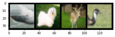
plot_images(images,labels)
print(' '.join('%5s' % d_idx2class[int(labels[j])]for j in range(len(images))))
ship dog deer bird
Making the CNN Link to heading
import torch.nn as nn
import torch.nn.functional as F
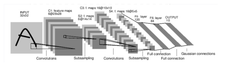
We’re going to define a class Net that has the CNN. This class will inherit from nn.Module and have two methods: an __init__() method and a forward() method. Here’s the architecture (except ours is on CIFAR, not MNIST):
Neural network components Link to heading
It looks like all layers run only for a batch of samples and not for a single point. The input to a nn.Conv2d layer for example will be something of shape (nSamples x nChannels x Height x Width), or (S x C x H x W).
If you want to put a single sample through, you can use input.unsqueeze(0) to add a fake batch dimension to it so that it will work properly.
Convolutional layers Link to heading
The first type of layer we have is a 2D convolutional layer, implemented using nn.Conv2d(). This has three compulsory parameters:
in_channels: basically the number of channels in your input data. For CIFAR we have 3 channels (RGB), for a dataset like MNIST we would only have one.out_channels: the number of convolutional filters you’d like to have in this layer. The network will learn the weights for all of these.kernel_size: the size of the square filter. Set to 3 to use 3x3 conv filters, 2 to use 2x2 conv filters etc.
There are also a bunch of other parameters you can set: stride, padding, dilation and so forth. This link has a good description of these parameters and how they affect the results.
MaxPooling layers Link to heading
These are called nn.MaxPool2d(). The compulsory parameter is kernel_size and it sets the size of the square window to which the maxpool operator is called. Like before you can set strides and other parameters.
Linear layers Link to heading
A simple linear layer of the form y = XW + b.
Parameters: in_features (neurons coming into the layer), out_features (neurons going out of the layer) and bias, which you should set to True almost always.
Activations Link to heading
We will use ReLu activations in the network. We can find that in F.relu and it is simple to apply. We’ll use the forward method to take layers we define in __init__ and stitch them together with F.relu as the activation function.
Reshaping Link to heading
If x is a Tensor, we use x.view to reshape it. For example, if x is given by a 16x1 tensor. x.view(4,4) reshapes it to a 4x4 tensor. You can write -1 to infer the dimension on that axis, based on the number of elements in x and the shape of the other axes. For example, x.view(2,-1) returns a Tensor of shape 2x8. Only one axis can be inferred.
The view function doesn’t create a new object. The object returned by view shares data with the original object, so if you change one, the other changes. This contrasts with np.reshape, which returns a new object.
class Net(nn.Module):
    def __init__(self):
        super().__init__()
        self.conv1 = nn.Conv2d(3, 6, 5)
        # we use the maxpool multiple times, but define it once
        self.pool = nn.MaxPool2d(2,2)
        # in_channels = 6 because self.conv1 output 6 channel
        self.conv2 = nn.Conv2d(6,16,5)
        # 5*5 comes from the dimension of the last convnet layer
        self.fc1 = nn.Linear(16*5*5, 120)
        self.fc2 = nn.Linear(120, 84)
        self.fc3 = nn.Linear(84, 10)

    def forward(self, x):
        x = self.pool(F.relu(self.conv1(x)))
        x = self.pool(F.relu(self.conv2(x)))
        x = x.view(-1, 16*5*5)
        x = F.relu(self.fc1(x))
        x = F.relu(self.fc2(x))
        x = self.fc3(x)  # no activation on final layer
        return x

net = Net()
Loss function and optimisation Link to heading
We will use a cross entropy loss, found in the function nn.CrossEntropyLoss(). This function expects raw logits as the final layer of the neural network, which is why we didn’t have a softmax final layer. The function also has a weights parameter which would be useful if we had some unbalanced classes, because it could oversample the rare class.
Optimisation is done with stochastic gradient descent, or optim.SGD. The first argument is the parameters of the neural network: i.e. you are giving the optimiser something to optimise. Second argument is the learning rate, and third argument is an option to set a momentum parameter and hence use momentum in the optimisation. Other options include dampening for momentum, l2 weight decay and an option for Nesterov momentum.
import torch.optim as optim

criterion = nn.CrossEntropyLoss()
optimizer = optim.SGD(net.parameters(), lr=0.001, momentum=0.9)
Note that nn.CrossEntropyLoss() returns a function, that we’ve called criterion, so when you see criterion later on remember it’s actually a function.
Training Link to heading
Let’s go through how to train the network.
A reminder: we’d defined trainloader like this:
trainloader = torch.utils.data.DataLoader(train, batch_size=4,
                                          shuffle=True, num_workers=2)
If we iterate through trainloader we get tuples with (data, labels), so we’ll have to unpack it. The variable data refers to the image data and it’ll come in batches of 4 at each iteration, as a Tensor of size (4, 3, 32, 32). labels will be a 1d Tensor.
Next we zero the gradient with optimizer.zero_grad(). Gradients aren’t reset to zero after a backprop step, so if we don’t do this, they’ll accumulate and won’t be correct.
Then comes the forward pass. We created an instance of our Net module earlier, and called it net. We can put an image through the network directly with net(inputs), which is the same as the forward pass.
Loss is easy: just put criterion(outputs, labels), and you’ll get a tensor back. Backpropagate with loss.backward(), and rely on the autograd functionality of Pytorch to get gradients for your weights with respect to the loss (no analytical calculations of derivatives required!)
Update weights with optimizer.step(). This uses the learning rate and the algorithm that you seeded optim.SGD with and updates the parameters of the network (that you also gave to optim.SGD)
Finally, we’ll want to keep track of the average loss. This will let us see if our network is learning quickly enough. We’ll print out diagnostics every so often.
running_loss = 0
printfreq = 1000
for epoch in range(2):
    for i, data in enumerate(trainloader):
        inputs, labels = data
        optimizer.zero_grad()
        outputs = net(inputs)  # forward pass
        loss = criterion(outputs, labels)
        loss.backward()
        optimizer.step()

        running_loss += loss.item()
        if i % printfreq == printfreq-1:
            print(epoch, i+1, running_loss / printfreq)
            running_loss = 0
0 1000 2.261470085859299
0 2000 1.9996697949171067
0 3000 1.8479941136837006
0 4000 1.735244540154934
0 5000 1.6975953910946846
0 6000 1.6573741003870963
0 7000 1.5628319020867347
0 8000 1.5547611890733242
0 9000 1.5162546570003033
0 10000 1.5124652062356472
0 11000 1.4926373654603957
0 12000 1.4613762157261372
1 1000 2.169555962353945
1 2000 1.4098796974420547
1 3000 1.4137214373350144
1 4000 1.3870477629005908
1 5000 1.351047681376338
1 6000 1.3671476569324732
1 7000 1.329134451970458
1 8000 1.32600463321805
1 9000 1.3019814370572567
1 10000 1.3028037322461605
1 11000 1.309966327637434
1 12000 1.2809565272629262
Saving, loading, and state_dict
Link to heading
It is good to save and load models. Models can take a long time to train, so saving them after they are done is good to avoid retraining them. You’ll also need a way to reload them.
When saving a model, we want to save the state_dict of the network (net.state_dict(), which holds weights for all the layers. This doesn’t save any of the optimiser information, so if we want to save that, we can also save optimiser.state_dict() too.
Let’s have a look in the state_dict of our net that we trained:
for param_tensor in net.state_dict():
    print(param_tensor, "\t", net.state_dict()[param_tensor].size())
conv1.weight 	 torch.Size([6, 3, 5, 5])
conv1.bias 	 torch.Size([6])
conv2.weight 	 torch.Size([16, 6, 5, 5])
conv2.bias 	 torch.Size([16])
fc1.weight 	 torch.Size([120, 400])
fc1.bias 	 torch.Size([120])
fc2.weight 	 torch.Size([84, 120])
fc2.bias 	 torch.Size([84])
fc3.weight 	 torch.Size([10, 84])
fc3.bias 	 torch.Size([10])
We can see the bias and weights are saved, each in the correct shape of the layer.
Let’s look at the state_dict of the optimiser object too:
print(optimizer.state_dict().keys())
print(optimizer.state_dict()['param_groups'])
dict_keys(['state', 'param_groups'])
[{'lr': 0.001, 'momentum': 0.9, 'dampening': 0, 'weight_decay': 0, 'nesterov': False, 'params': [5019782816, 5019782960, 5019782600, 5019782672, 5019782888, 5019781736, 5019782456, 5019779720, 5019781592, 5019779792]}]
There’s more, but it’s big, so I won’t print it.
Saving and loading is done with torch.save, torch.load, and net.load_state_dict. Saving an object will pickle it. It seems to be a PyTorch convention to save the weights with a .pt or a .pth file extension.
fname = './models/CIFAR10_cnn.pth'
torch.save(net.state_dict(), fname)
loaded_dict = torch.load(fname)
net.load_state_dict(loaded_dict)
<All keys matched successfully>
Some layers like Dropout or Batchnorm won’t work properly if you don’t call net.eval() after loading.
net.eval()
Net(
  (conv1): Conv2d(3, 6, kernel_size=(5, 5), stride=(1, 1))
  (pool): MaxPool2d(kernel_size=2, stride=2, padding=0, dilation=1, ceil_mode=False)
  (conv2): Conv2d(6, 16, kernel_size=(5, 5), stride=(1, 1))
  (fc1): Linear(in_features=400, out_features=120, bias=True)
  (fc2): Linear(in_features=120, out_features=84, bias=True)
  (fc3): Linear(in_features=84, out_features=10, bias=True)
)
There is much more to saving and loading than this. Check out this guide for more information. Some examples: transfer learning, model checkpointing, transferring from CPU to GPU and vice versa.
Model testing Link to heading
It’s time to see how our trained net does on the test set. Will it have learned anything?
# Reload net if needed
fname = './models/CIFAR10_cnn.pth'
loaded_dict = torch.load(fname)
net.load_state_dict(loaded_dict)
<All keys matched successfully>
As a sanity check, let’s first take some images from our test set and plot them with their ground-truth labels:
dataiter = iter(testloader)
images, labels = dataiter.next()
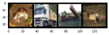
plot_images(images,labels)
print(' '.join('%5s' % d_idx2class[int(labels[j])]for j in range(len(images))))
frog truck truck deer

Looks good. Now let’s run the images through our net and see what we get.
outputs = net(images)
print(outputs)
tensor([[-2.4268, -2.2433,  0.7154,  1.9097,  2.9379,  1.5184,  1.5930,  0.7512,
         -3.0894, -3.7157],
        [ 2.6312,  2.0198, -0.4813, -1.5693, -2.4001, -2.0169, -4.2537,  0.2893,
          2.6629,  3.0607],
        [ 1.0008,  0.0441, -1.0073, -0.1218, -0.4955, -1.1580, -1.8499, -0.0223,
          1.5421,  1.3126],
        [-1.0473, -2.0484,  0.8610,  0.7433,  4.1755,  0.5730,  2.4846, -0.3962,
         -2.6474, -3.2877]], grad_fn=<AddmmBackward>)
These are logits for each of the ten classes. Since the highest logit will be the predicted class, we can generate labels easily from the logits.
preds = outputs.argmax(dim=1)
plot_images(images,preds)
print(' '.join('%5s' % d_idx2class[int(preds[j])]for j in range(len(images))))
deer truck ship deer
It’s got some right, not all. For a better evaluation of performance, we’ll have to look at performance across the entire test set.
Most of the code follows similar patterns to the training loop above. I’ll comment on the things I find interesting.
A useful function is torch.max(). This returns a namedtuple with the standard max values along an axis, but somewhat usefully also the argmax values along that axis, too. This is good for us because we don’t really care about the max value, but more its argmax, since that corresponds to the label.
We can do element-wise comparison with == on PyTorch tensors (and Numpy arrays too). We see this in the line using predicted == labels below, which will return a vector filled with True/False values. If predicted and labels were lists, by comparison, we’d just get a single True value if all the elements were the same, or False if any were different.
`
Note the code is inside the torch.no_grad() context manager, which turns off gradient tracking for the variables. It’s claimed that this reduces memory usage, and increases computation speed. I wasn’t sure, so I did a rudimentary speed test. I didn’t track the memory usage, but there is definitely a speed benefit.
Results:
- with
no_grad(): 50.8 s - without
no_grad(): 55.6s
Given it’s one line, it’s probably worth the effort to do.
total = 0  # keeps track of how many images we have processed
correct = 0  # keeps track of how many correct images our net predicts
with torch.no_grad():
    for i, data in enumerate(testloader):
        images, labels = data
        outputs = net(images)
        _, predicted = torch.max(outputs.data, 1)
        total += labels.size()[0]
        correct += (predicted == labels).sum().item()

print("Accuracy: ", correct/total)
Accuracy: 0.56358
We are tracking at about 56% accuracy.
Prediction analysis Link to heading
We’re going to want to know how our model does on different classes. It’s unlikely its predictions for every class will be similarly accurate.
class_correct = list(0 for i in range(10))  # Holds how many correct images for the class
class_total = list(0 for i in range(10))  # Holds total images for the class

with torch.no_grad():
    for i, data in enumerate(testloader):
        images, labels = data
        outputs = net(images)
        _, predicted = torch.max(outputs, 1)
        c = (predicted == labels)
        for j in range(4):
            label = labels[j]
            class_correct[label] += c[j].item()
            class_total[label] += 1

for i in range(10):
    print('Accuracy of %5s : %2d %%' % (
        d_idx2class[i], 100 * class_correct[i] / class_total[i]))
Accuracy of airplane : 69 %
Accuracy of automobile : 69 %
Accuracy of  bird : 35 %
Accuracy of   cat : 44 %
Accuracy of  deer : 60 %
Accuracy of   dog : 33 %
Accuracy of  frog : 57 %
Accuracy of horse : 73 %
Accuracy of  ship : 73 %
Accuracy of truck : 46 %
You can see significant differences in the accuracy of different classes. For example, our network is bad at predicting birds, but better at predicting horses.