Sarsa, expected sarsa and Q-learning on the OpenAI taxi environment
In this post, we’ll see how three commonly-used reinforcement algorithms - sarsa, expected sarsa and q-learning - stack up on the OpenAI Gym Taxi (v2) environment.
Note: this post assumes that the reader is familiar with basic RL concepts. A good resource for learning these is the textbook by Sutton and Barto (2018), which is freely available online.
Sarsa, Expected Sarsa and Q-Learning Link to heading
So, what are these algorithms?
Let’s say our agent is currently at state s, and takes action a. Our action-value function, q(s,a), gives us an estimate for how good this was for the agent. Initially this is set to 0, since our agent doesn’t know anything yet. We’ll need to update this function as our agent learns more about its environment.
The algorithms are similar, in that they all update q(s,a) after every time step. They do this by using information about the next reward $R_{t+1}$, and the action-value function for the next state and action, q(s’,a’).
The algorithms are different in the exact way q(s,a) is updated. Each algorithm agrees that the agent ends up at s’, but disagrees as to how to calculate the value of the next state, q(s’,a’).
According to Sarsa, once the agent gets to s’, it will follow its policy, $ \pi$. Knowing this information, we can sample an action a’ from $ \pi$ at state s’, and use q(s’, a’) as the estimate of the next state:
$$ q(s,a) = q(s,a) + \alpha \left[ R_{t+1} + \gamma q(s’, a’) - q(s,a) \right]$$
Expected Sarsa, on the other hand, reasons that rather than sampling from $\pi$ to pick an action a’ by, we should just calculate the expected value of s’. This way, the estimate of how good s’ is won’t fluctuate around, like it would when sampling an action from a distribution, but rather remain steady around the “average” outcome for the state.
$$ q(s,a) = q(s,a) + \alpha \left[ R_{t+1} + \gamma \sum_{a’} \pi (a’ | s’) q(s’, a’) - q(s,a) \right] $$
Q-learning takes a different approach. It assumes that when the agent is in state s’, it will take the action a’ that it thinks is the best action. In other words, it will take the action a’ that maximises q(s’, a’).
$$ q(s,a) = q(s,a) + \alpha \left[ R_{t+1} + \gamma \max_{a’} q(s’, a’) - q(s,a) \right] $$
So how differently do these algorithms perform? Let’s find out by using the Taxi environment in the OpenAI Gym.
OpenAI Gym Taxi Environment Link to heading
A taxi in its 5x5 environment
In this environment, the agent operates a taxi that must pick up and drop off passengers in a 5x5 grid.
The taxi can move in four directions: north, south, east and west. Passengers are picked up from one of four locations and then must be dropped off at their destination.
The taxi can take the following actions (numbering same as in the environment):
- 0: move south
- 1: move north
- 2: move east
- 3: move west
- 4: pick up passenger
- 5: drop off passenger
The agent recieves a reward of -1 on every timestep, and an additional reward of +20 for delivering the passenger. Attempting to pick up or drop off the passenger illegally gives a reward of -10.
An episode is finished either when a passenger completes their journey or after 200 time steps; whatever is sooner.
Creating the agent Link to heading
First thing to do is import all the libraries we’ll need:
import gym
import numpy as np
import pandas as pd
import matplotlib.pyplot as plt
%matplotlib inline

# For animation
from IPython.display import clear_output
from time import sleep
We’re going to create a class called Agent. The idea is that we can specify a single parameter, method, and use that to determine which algorithm the agent uses to learn.
Our class starts like this.
class Agent:
    def __init__(self, method):
        pass

    def simulate_episode(self):
        pass
Let’s look at the init() method first. In this method we’ll initialise environment parameters, like the number of squares the taxi can go in, or the number of actions the taxi can take. We’ll also set up the initial values for parameters $ \alpha$, $ \gamma$ ,$ \epsilon$, initialise our table of q-values and create our policy, which starts off as the equiprobable random policy.
Oh, and we’ll also define which environment we’d like to use. That’s what the line self.env = gym.make('Taxi-v2') does below.
def __init__(self, method, start_alpha = 0.3, start_gamma = 0.9, start_epsilon = 0.5):
    """method: one of 'q_learning', 'sarsa' or 'expected_sarsa' """
    self.method = method
    self.env = gym.make('Taxi-v2')
    self.n_squares = 25
    self.n_passenger_locs = 5
    self.n_dropoffs = 4
    self.n_actions = self.env.action_space.n
    self.epsilon = start_epsilon
    self.gamma = start_gamma
    self.alpha = start_alpha
    # Set up initial q-table
    self.q = np.zeros(shape = (self.n_squares*self.n_passenger_locs*self.n_dropoffs, self.env.action_space.n))
    # Set up policy pi, init as equiprobable random policy
    self.pi = np.zeros_like(self.q)
    for i in range(self.pi.shape[0]):
        for a in range(self.n_actions):
            self.pi[i,a] = 1/self.n_actions
Next we’ll create our function that runs an episode of the environment. I’ll put the code up here, then run through it below.
def simulate_episode(self):
    s = self.env.reset()
    done = False
    r_sum = 0
    n_steps = 0
    gam = self.gamma
    while not done:
        n_steps += 1
        # take action from policy
        x = np.random.random()
        a = np.argmax(np.cumsum(self.pi[s,:]) > x)
        # take step
        s_prime,r,done,info = self.env.step(a)
        if self.method == 'q_learning':
            a_prime = np.random.choice(np.where(self.q[s_prime] == max(self.q[s_prime]))[0])
            self.q[s,a] = self.q[s,a] + self.alpha * \
                (r + gam*self.q[s_prime,a_prime] - self.q[s,a])
        elif self.method == 'sarsa':
            a_prime = np.argmax(np.cumsum(self.pi[s_prime,:]) > np.random.random())
            self.q[s,a] = self.q[s,a] + self.alpha * \
                (r + gam*self.q[s_prime,a_prime ] - self.q[s,a])
        elif self.method == 'expected_sarsa':
            self.q[s,a] = self.q[s,a] + self.alpha * \
                (r + gam* np.dot(self.pi[s_prime,:],self.q[s_prime,:]) - self.q[s,a])
        else:
            raise Exception("Invalid method provided")
        # update policy
        best_a = np.random.choice(np.where(self.q[s] == max(self.q[s]))[0])
        for i in range(self.n_actions):
            if i == best_a:      self.pi[s,i] = 1 - (self.n_actions-1)*(self.epsilon / self.n_actions)
            else:                self.pi[s,i] = self.epsilon / self.n_actions

        # decay gamma close to the end of the episode
        if n_steps > 185:
            gam *= 0.875
        s = s_prime
        r_sum += r
    return r_sum
s = self.env.reset() is used to start a new episode. It resets the environment, placing the car in a random position and randomising the passenger/dropoff locations. The state that we start in is saved under the variable s.
Next we initialise our variables to update. The episode will end when done is set to True. The variable r_sum holds a running reward sum from the episode, and n_steps is used to track when we are getting close to the end of the episode. We also initialise gam = self.gamma . We want to decay gamma, the discount factor for future rewards, towards the end of the episode once we don’t have many time steps left.
Now we come to the actual episode itself. In each time step, we sample an action from our policy pi: a = np.argmax(np.cumsum(self.pi[s,:]) > np.random.random()) , and then use s_prime,r,done,info = self.env.step(a) to make the action, collect the reward, record the next state and check if the episode is finished (note: s_prime refers to s’ ).
At this point we update the estimate for q(s,a) and how we update it differs according to what method we are using. These lines of code just implement the equations from the first part of the post - not super interesting, really, but of great potential impact for learning our policy.
Next, it’s time to update our policy pi. That’s this bit of code:
best_a = np.random.choice(np.where(self.q[s] == max(self.q[s]))[0])
for i in range(self.n_actions):
    if i == best_a:      self.pi[s,i] = 1 - (self.n_actions-1)*(self.epsilon / self.n_actions)
    else:                self.pi[s,i] = self.epsilon / self.n_actions
First we find what the best action is for our current state. That is, if the agent is in state s, what a gives the highest q(s,a)? This is what best_a represents above.
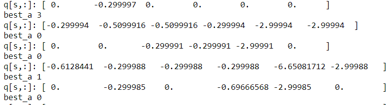
A printout of some states and their q-values. The best action is the one that maximises q(s,a). If there’s a tie, it’s better to split randomly.
Once we know the best action, we update the policy. We want to pick the best action with $ 1 - \epsilon$ chance and choose randomly with $ \epsilon$ chance. The if/else statement implements these probabilities.
Next we decay gamma a bit, but only if we’re close to the end of the episode. This is because with just a few time periods left, there should be more incentive for short-term behavior because long-term actions don’t have time to pay off. Finally, the reward is added to the reward sum and the state rolled forward.
Training the agent Link to heading
Here’s the code for training the agent, where we run lots of episodes in which the agent attempts to maximise its reward. We know that the Taxi environment will not change over time, so if the policy and action-value functions stabilise there isn’t any problem for us.
def train_agent(agent, n_episodes= 200001, epsilon_decay = 0.99995, alpha_decay = 0.99995, print_trace = False):
    r_sums = []
    for ep in range(n_episodes):
        r_sum = agent.simulate_episode()
        # decrease epsilon and learning rate
        agent.epsilon *= epsilon_decay
        agent.alpha *= alpha_decay
        if print_trace:
            if ep % 20000 == 0 and ep > 0 :
                print("Episode:", ep, "alpha:", np.round(agent.alpha, 3), "epsilon:",  np.round(agent.epsilon, 3))
                print ("Last 100 episodes avg reward: ", np.mean(r_sums[ep-100:ep]))
        r_sums.append(r_sum)
    return r_sums
We start by initialising r_sums, a container that will hold the reward sum r_sum of every episode. Then we run the episode, and decrease epsilon and alpha after each episode. Why?
Decreasing epsilon (our exploration parameter) over time makes sense. Each episode, the agent becomes more and more confident what good and bad choices look like. Decreasing epsilon is required if we seek to maximise our reward sum, since exploratory actions typically aren’t optimal actions, and besides, we can be fairly sure what are good actions and bad actions by this point anyway. There is a similar argument for decreasing alpha (the learning rate) over time - we don’t want the estimates to jump around too much once we are confident in their validity.
Now we can create our agents and train them.
# Create agents
sarsa_agent = Agent(method='sarsa')
e_sarsa_agent = Agent(method='expected_sarsa')
q_learning_agent = Agent(method='q_learning')

# Train agents
r_sums_sarsa = train_agent(sarsa_agent, print_trace=True)
r_sums_e_sarsa = train_agent(e_sarsa_agent, print_trace=True)
r_sums_q_learning = train_agent(q_learning_agent, print_trace=True)
Which method is best? Link to heading
After training our agents we can compare their performance to each other. The criteria for comparison we’ll use is the best 100-epsiode average reward for each agent.
Let’s plot the 100-epsiode rolling cumulative reward over time:
df = pd.DataFrame({"Sarsa": r_sums_sarsa,
             "Expected_Sarsa": r_sums_e_sarsa,
             "Q-Learning": r_sums_q_learning})
df_ma = df.rolling(100, min_periods = 100).mean()
df_ma.iloc[1:1000].plot()
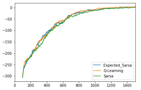
The green line (sarsa) seems to be below the others fairly consistently, but it’s close.
Looks like the Sarsa agent tends to train slower than the other two, but not by a whole lot. At the end of 200000 episodes, however, it’s Expected Sarsa that’s delivered the best reward:
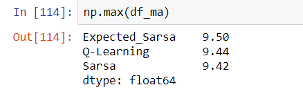
The best 100-episode streak gave this average return. Expected Sarsa comes out on top, but all three agents are close.
A 100-episode average reward of 9.50 isn’t too bad at all. In fact, it would put us on the leaderboard for this problem!
Viewing the policy Link to heading
It can be quite tricky to understand the difference between agents. Even if one agent does better than the other two, it isn’t straightforward to see the reasons why.
Visualising the policy is one way to find out. Here’s some code to render the environment and to see how the agent behaves. (credit to these guys.)
def generate_frames(agent, start_state):
agent.env.reset()
agent.env.env.s = start_state
s = start_state
policy = np.argmax(agent.pi,axis =1)
epochs = 0
penalties, reward = 0, 0
frames = []
done = False
frames.append({
'frame': agent.env.render(mode='ansi'),
'state': agent.env.env.s ,
'action': "Start",
'reward': 0
}
)
while not done:
a = policy[s]
s, reward, done, info = agent.env.step(a)
if reward == -10:
penalties += 1
# Put each rendered frame into dict for animation
frames.append({
'frame': agent.env.render(mode='ansi'),
'state': s,
'action': a,
'reward': reward
}
)
epochs += 1
print("Timesteps taken: {}".format(epochs))
print("Penalties incurred: {}".format(penalties))
return frames
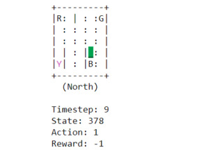
def print_frames(frames):
for i, frame in enumerate(frames):
clear_output(wait=True)
print(frame['frame'].getvalue())
print(f"Timestep: {i + 1}")
print(f"State: {frame['state']}")
print(f"Action: {frame['action']}")
print(f"Reward: {frame['reward']}")
sleep(.4)
Below we demonstrate some differences in policy between the expected sarsa agent and the sarsa agent. While the expected sarsa agent has learned the optimal policy, the sarsa agent hasn’t yet - but it’s not far off. (Note: these policies are before the agent is fully trained (after around 15000 episodes)).
Expected Sarsa
Sarsa
Conclusion Link to heading
The three agents seemed to perform around the same on this task, with Sarsa being a little worse than the other two. This result doesn’t always hold - on some tasks (see “The Cliff” - Sutton and Barto (2018)) they perform very differently, but here the results were similar. It would be interesting to see how a planning / n-step algorithm would perform on this task.