Let's build a DQN: basics
In February 2015, Google Brain published a paper combining deep neural networks and reinforcement learning for the first time - called DQN (deep q-network). It was a landmark moment.
DQN was the first algorithm that could successfully play a wide range of Atari games. Other algorithms at the time could perform well at a single game but couldn’t generalise across games. Impressively, DQN was able to perform above human level at a range of Atari games using only the screen pixels as input. Because it didn’t require any game-specific modifications to perform well at a game, DQN was heralded as a key breakthrough towards artificial general intelligence.
In this post, I will go through some of the basic theory of DQNs. In the next post we’ll code up a basic DQN on the cartpole problem and see some of the limitations of the basic model. After that, we’ll make some changes to improve the performance of the model and see how it goes on a more complicated environment.
The DQN algorithm is not hard to understand, but I found it easiest to comprehend when broken down into concepts. Together, the concepts chunk together to form a cohesive picture.
Concept 1: Q-learning Link to heading
Q-learning deserves an entire post for itself, and luckily many have already been written. The “RL bible” by Sutton and Barto gives a great overview of q-learning, or for a quicker overview, try this nice introduction. If you’d like more, move on to implementing q-learning with the OpenAI gym.
I’ll assume you know about q-learning and reinforcement learning basics for the rest of this post.
When we use q-learning with a discrete state space, we typically use a table to store the q-value for each state. This is called a q-table.
The q-table provides an “expected reward” for each action the agent can take in a state. This is useful because a) it allows the agent to identify which actions are the strongest, and b) it provides a convenient way to update the q-estimate of a state (which is where q-learning comes in).
Concept 2: Continuous space Link to heading
But, a q-table only works with a discrete state space, or when the agent can only be in a set number of states.
Think a grid. A maze. A card game. Not the movements of a robot. Not for a racecar going around a track. Not for Dota or Starcraft 2.
To illustrate some situations where a q-table can be used, we can look at the toy-text OpenAI gym environments. For example:
- Taxi-v2: The agent is confined to a 5x5 grid, there are 5 possible passenger locations, and 4 passenger dropoff locations - making 500 possible states.
- GuessingGame-v0: there are only four possible states: no guess yet, guess too low, guess too high, guess correct
- Blackjack-v0: states are made up of the combinations of the players current card sum, the faceup card of the dealer, and if the player has a useable ace.
By contrast, none of the classic control environments have a discrete state space. The following quantities are all continuous:
- CartPole-v1: state is made up of cart position, cart velocity, pole angle, and pole velocity at tip
- MountainCar-v0: state is car position and car velocity
- Acrobot-v1: state is the sin and the cos of the two rotational joint angles, and the joint angular velocities.
Why not use a q-table when your state is continuous? Answer: you can’t.
The first problem is that there are too many states to store in the table. The q-table could very easily have more than a billion records. The immense memory requirements quickly torpedo your chances at finding a solution. It’d also be really, really slow to train.
The second problem is that a q-table assumes that each state is independent of each other. This clearly isn’t true for continuous environments. Many states are very similar to each other, and we’d like our agent to behave similarly in those states. In other words – if our agent learns something in one state, it should generalise the knowledge to other similar states. This isn’t possible with a q-table.
So, we need a new approach.
Concept 3: Approximating neural network Link to heading
What if we represented the q-values of each state with a model? Something where we could give as input our state and get as output the q-value for that state.
This is like a regression problem. We have a bunch of labelled data points. The q-value is the thing we’re trying to model (the y-variable, response variable, dependent variable), given the state (x-variables, independent variables, explanatory variables).
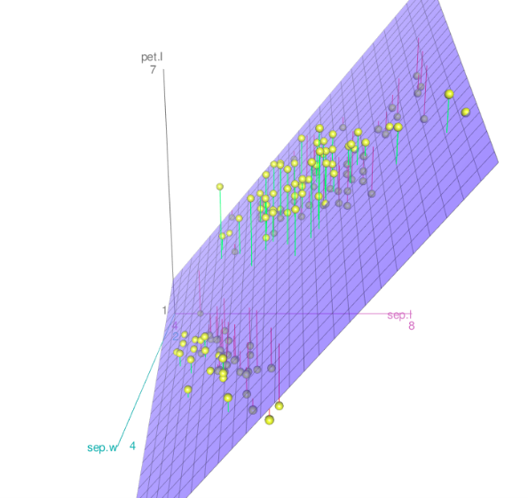
In other words, we want to make a n-dimensional surface that fits our q-values. You might see this described as a q-surface.
We could use a hyperplane, a linear surface that fits the points. That could have some advantages.
A linear surface fitting some points
But many environments are too complex for a linear surface. It’d be useful to go non-linear.

An example non-linear q-surface for an environment
There are many ways to make a non-linear surface, but the most popular way is with a neural network. That’s what DQN uses.
Concept 4: Instability Link to heading
Let’s say we’ve created a neural network, with some number of hidden layers. I’ll assume that you know what a neural network is and (roughly) how it works.
Each neuron has a bias term, b, and each link between the neurons has a weight, w.
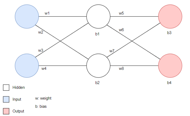
A neural network with two input neurons, two neurons in the hidden layer, and two output neurons.
We can put those weights and biases together into a vector, w, and say that w parameterises the neural network. In other words, the values of w determine how our neural network acts.
We want to modify w so that the neural network forms a good approximation for our action-value function, q(s,a). If this were a straightforward supervised learning task, we’d use gradient descent and backpropagation to slowly adjust the values of w until we reach a (possibly local) optimum.
But there is a twist. For traditional supervised learning tasks, we are trying to fit a surface to a bunch of points, which are the true values of the observations. For reinforcement learning tasks, we are also trying to fit a surface to some points, except that our points are estimates of the true values of the observations. That means the points tend to move around.
Why do the points move around? Remember that the points represent the action-value function, q(s,a). While the true value of a state-action pair is a fixed value, we don’t know what that true value is - we just have an estimate for the value. Our estimates (obtained using q-learning) will improve over time as the agent collects more information, but they will jump around in the process.
Normally with gradient descent, we converge over time to an optimal solution, or at least a locally optimal solution. Each step brings us closer and closer to our ideal surface. But that assumes the points don’t change.
If we are fitting a surface to a bunch of points, and the points are also moving around, the gradient descent procedure is going to have problems. Imagine you’re playing golf, and every time you hit the ball towards the hole, the hole changed location – three hundred metres to the right, one hundred to the left, twelve metres behind you. You wouldn’t make much progress. It’s similar to what happens with gradient descent when its target changes.
Let’s call our true value of the action-value function q(s,a) , and our estimate for the state U . It turns out that if U is an unbiased estimate for q(s,a) , then gradient descent will eventually converge on the best solution. If U isn’t an unbiased estimate, then no such guarantees apply.
For q-learning, U isn’t an unbiased estimate. Say you are in state s , you take action a , and you end up in state s’ . The target of the q-learning update, $ \max_{a’} q(s’,a’)$ - depends on the weights w of the approximating neural network. But you are also performing gradient descent on w, trying to iterate them towards an ideal solution. This means that the gradient descent process can suffer from oscillations or even diverge away from the optimal values.
To conclude: there’s no guarantee that the neural network will converge to the ideal solution. In fact, we are likely to end up with an unstable solution.
Luckily, there are some improvements we can make.
Instability improvement 1: Minibatch training Link to heading
So far, we perform gradient descent after each action. We use the current <s, a, r, s’> (state, action, reward, next state) tuple to run the gradient descent on each observation as we get them. This is known as stochastic gradient descent.
It turns out this isn’t a particularly good way of doing things. We can increase the speed and accuracy of our gradient descent updates by using information from n data points at once selected randomly – called a minibatch. This makes the gradient descent updates are smoother and more accurate as you can estimate the gradient update from a sample of n data points, rather than just from one data point.
The image below (source) shows a good demonstration of this.
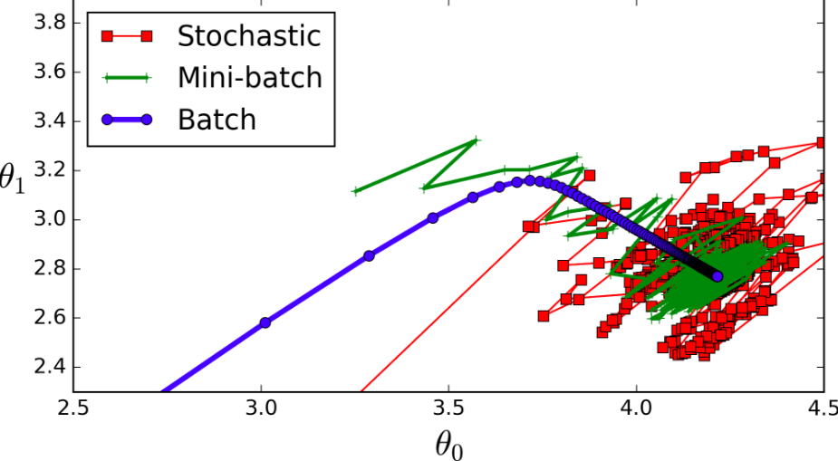
Weight updates for a sample gradient descent task.
The red line makes a step after encountering every data point, and it moves all over the place. The green line uses information from some number of data points (a “minibatch”) to make a move, yielding a smoother descent to the optimum value. The blue line uses the entire dataset (a “batch”) to make a gradient descent update and is the smoothest of all three lines. Unfortunately batch gradient descent is not possible in reinforcement learning tasks because a) the entire dataset is not available, and b) we want to learn as the agent collects it (online learning).
Instability improvement 2: Experience replay Link to heading
To use minibatch gradient descent, we’ll need multiple data points to train off. In other words, we’ll store each sequence of <s,a,r,s’> in a list as we get them. Now we can use the last n (32 is a common size) data points in our mini-batch gradient descent.
This is good, because our agent can learn from the same experience multiple times, which is more efficient than just learning from it once. Using minibatch training also makes the gradient descent procedure smoother and quicker.
But, rather than performing an online q-learning update on whatever <s,a,r, s’> tuple the agent is up to, it’d be better to instead sample randomly from the past experiences of the agent.
If we don’t sample randomly, the gradient descent updates use the recent experiences of the agent - experiences which are naturally highly correlated with each other. We can reduce this correlation by sampling randomly, which means the weights w of the neural network don’t influence the training procedure quite as much - leading to reduced instability.
That’s the basic theory done – in the next post we’ll code up the algorithm and see how it goes on the CartPole environment.
I’d also like to pay homage to this series on DQN’s. It was this resource that really made the algorithm click for me - check it out if you’re having trouble following anything here as I’ve written it.