Let's build a DQN: simple implementation
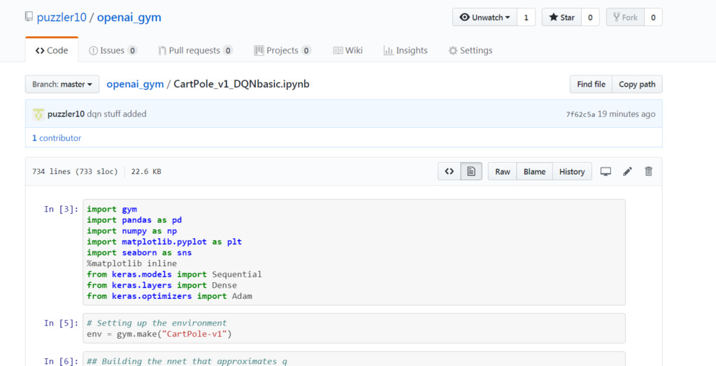 Click the image above to see the source code.
Last time, we established some theory for our DQN. Now it’s time to implement it.
We won’t build a full DQN from the DeepMind paper, not yet. Instead we’ll build a simplified version. I call it the basic DQN.
The basic DQN is the same as the full DQN, but missing a target network and reward clipping. We’ll get to that in the next post.
We use the OpenAI gym, the CartPole-v1 environment, and Python 3.6. Let’s get started.
Setup Link to heading
As usual, first thing is to import libraries:
# General
import gym
import pandas as pd
import numpy as np
# Neural network
from keras.models import Sequential
from keras.layers import Dense
from keras.optimizers import Adam
# Plotting
import matplotlib.pyplot as plt
import seaborn as sns
%matplotlib inline
We then set up the environment with the gym.make() command.
env = gym.make("CartPole-v1")
Approximating q(s,a) with a neural network Link to heading
The DQN is for problems that have a continuous state, not a discrete state. That rules out the use of a q-table.
Instead we build a neural network to represent q. There are many ways to build a neural network. I choose keras.
This neural network will map the state, s (usually a vector) to the possible actions, a.
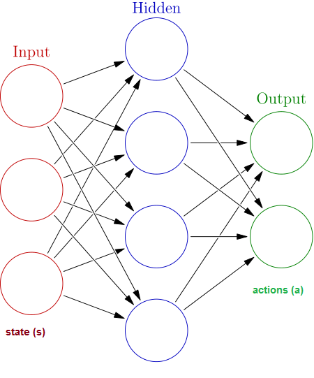
One input neuron for every component of the state vector. One output neuron for every possible action.
Say the above neural network represented the q-function. Our state would be a vector of length three. Examples? X, Y and Z position for a game, or card sum, dealer faceup card and useable ace for blackjack.
We don’t need a complicated neural network structure for our problem. A network with one hidden layer will be fine. The environment dictates the number of input and output neurons in our network. Activation functions are relu, except for a linear output layer. Using the Adam optimiser lets us avoid choosing a learning rate.
## Building the nnet that approximates q
n_actions = env.action_space.n  # dim of output layer
input_dim = env.observation_space.shape[0]  # dim of input layer
model = Sequential()
model.add(Dense(64, input_dim = input_dim , activation = 'relu'))
model.add(Dense(32, activation = 'relu'))
model.add(Dense(n_actions, activation = 'linear'))
model.compile(optimizer=Adam(), loss = 'mse')
Parameters Link to heading
Next we initiate parameters:
n_episodes: how many episodes to rungamma: the discount factor that applies to rewardsepsilon: the exploration parameter: will decline over time.minibatch_size: how many <s,a,r,s’> experiences to include each time we update the q neural networkr_sums: list to store the reward from each episodereplay_memory: list to hold the <s,a,r,s’> experiencesmem_max_size: once thereplay_memorylist gets longer than this, overwrite old samples with new ones
Here’s some values for these parameters. Many different parameter values may work. Use hyperparameter tuning if you want to find the best ones.
n_episodes = 1000
gamma = 0.99
epsilon = 1
minibatch_size = 32
r_sums = []  # stores rewards of each epsiode
replay_memory = [] # replay memory holds s, a, r, s'
mem_max_size = 100000
Interaction Link to heading
for n in range(n_episodes):
    s = env.reset()
    done=False
    r_sum = 0
    while not done:
        # Uncomment this to see the agent learning
        # env.render()

        # Feedforward pass for current state to get predicted q-values for all actions
        qvals_s = model.predict(s.reshape(1,4))
        # Choose action to be epsilon-greedy
        if np.random.random() < epsilon:  a = env.action_space.sample()
        else:                             a = np.argmax(qvals_s);
        # Take step, store results
        sprime, r, done, info = env.step(a)
        r_sum += r
        # add to memory, respecting memory buffer limit
        if len(replay_memory) > mem_max_size:
            replay_memory.pop(0)
        replay_memory.append({"s":s,"a":a,"r":r,"sprime":sprime,"done":done})
        # Update state
        s=sprime
        # Train the nnet that approximates q(s,a), using the replay memory
        model=replay(replay_memory, minibatch_size = minibatch_size)
        # Decrease epsilon until we hit a target threshold
        if epsilon > 0.01:      epsilon -= 0.001
    print("Total reward:", r_sum)
    r_sums.append(r_sum)
We need to reset the environment each time we reach the end of an episode. That’s what env.reset() does.
Let’s go inside the inner loop. Say the agent is in a state s.
First the agent needs to know what the q-value is for each action in state s. Get this with the neural network’s predict method.
The agent then has to select an action. It could take the action with the highest q-value, or it could move randomly. It’s up to the epsilon parameter to determine how often each should happen.
The agent then executes its action. It ends up in s’ (sprime) and gets a reward r. Now the agent has a <s,a,r,s’> experience. We’ll also add the variable done to know if the episode has finished, making <s,a,r,s’,done>. Our experience replay function will use these experiences.
Time to add it to the memory. The memory can only hold mem_max_size elements. If our memory is full, we’ll ditch the oldest entry and replace it with the latest experience.
After, we train the q neural network using a minibatch_size amount of <s,a,r,s’,done> experiences. We’ll write a function called replay() to do this.
Finally we decrease epsilon a little. As the agent learns more about the environment it should explore less, until it hits a threshold.
The experience replay function Link to heading
Time to write the replay() function used earlier. This function trains our neural network that approximates q.
def replay(replay_memory, minibatch_size=32):
    # choose <s,a,r,s',done> experiences randomly from the memory
    minibatch = np.random.choice(replay_memory, minibatch_size, replace=True)
    # create one list containing s, one list containing a, etc
    s_l =      np.array(list(map(lambda x: x['s'], minibatch)))
    a_l =      np.array(list(map(lambda x: x['a'], minibatch)))
    r_l =      np.array(list(map(lambda x: x['r'], minibatch)))
    sprime_l = np.array(list(map(lambda x: x['sprime'], minibatch)))
    done_l   = np.array(list(map(lambda x: x['done'], minibatch)))
    # Find q(s', a') for all possible actions a'. Store in list
    # We'll use the maximum of these values for q-update
    qvals_sprime_l = model.predict(sprime_l)
    # Find q(s,a) for all possible actions a. Store in list
    target_f = model.predict(s_l)
    # q-update target
    # For the action we took, use the q-update value
    # For other actions, use the current nnet predicted value
    for i,(s,a,r,qvals_sprime, done) in enumerate(zip(s_l,a_l,r_l,qvals_sprime_l, done_l)):
        if not done:  target = r + gamma * np.max(qvals_sprime)
        else:         target = r
        target_f[i][a] = target
    # Update weights of neural network with fit()
    # Loss function is 0 for actions we didn't take
    model.fit(s_l, target_f, epochs=1, verbose=0)
    return model
Start off by selecting some entries randomly from our memory to form our minibatch. Select the samples without replacement.
Next we create one list to hold each s element, one list to hold each a element, one list to hold each r element, and so on. We’ll use these lists later on.
Now we find the action a’ that maximises q(s’,a’). We can use the predict() function of our neural network. Remember, by inputting the state s’ on one end, we get the q-estimate for every action. Now we know the best q-value for the state s’.
We eventually will need to train our neural network with some labelled <s, a> pairs. Our input to the neural network needs to be the same dimensions as s, and we need one value for every action. Remember this diagram?
We don’t know how good the other actions were. We didn’t take them – but we need a q-value for these actions anyway. What do we do?
Solution: use the current predicted values of the q-network for these actions. We can get these with target_f = model.predict(s_l). The loss function will be 0 for these since we have a perfect fit.
Now we need to add the q-estimate for the action the agent took. We do this with the q-learning update. We also need to split between the cases where the episode is already finished or not. If done=True then there is no next state to go to – the target is r. Else the q-update gives the target. Use the target to overwrite the predicted values for the action the agent took. Do this with the target_f vector.
Finally train the model using the minibatch. We don’t loop through the elements one by one and train on each of them. We train on all the elements at once and get the benefits of minibatch training.
Performance Link to heading
This environment is considered solved by getting an average reward of 475 over 100 episodes. The basic DQN can do this in xx episodes. How do we go? Here’s the results for 2500 episodes:
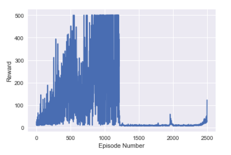
The basic DQN works pretty well. It learns how to balance the pole. It even gets quite good at it. But then it forgets what it knows. The performance becomes terrible. Eventually it will relearn how to balance the pole and the performance will return to high levels. We can see evidence of this towards the final episodes.
Why does this happen? The agent becomes successful at the task. The pole is balanced and the agents memory only has these experiences. This agent then uses this data for training. It then loses skills for when the pole isn’t already balanced. The memory starts to have more diverse experiences again. The agent starts to perform better.
This forgetting and relearning seems to be a constant feature for the DQN algorithm. Both the basic and full DQNs have this problem, called catastrophic forgetting. See this thread or this paper for more details.